MS Excel Worksheet
We offer you a brighter future with industry-ready online courses - Start Now!!
Excel worksheet comprises rows, columns, and cells. Each box in a worksheet is termed to be a cell. Excel Worksheet is also known as a spreadsheet. It is widely used to save data in a tabular form.
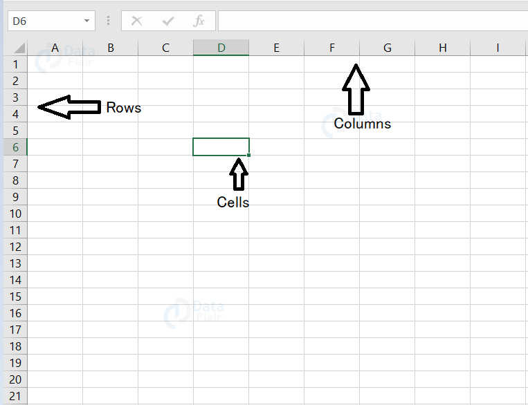
A worksheet in excel is a combination of cells where you enter, hold, and modify the data. The user can rename the worksheet and the worksheet helps in performing calculations. The worksheet is the place where the user stores the data, information. By default, the names of the worksheets are “Sheet 1”, “Sheet 2”, “Sheet 3”.
Click on the worksheet name to go to any worksheets.
When you click on the excel worksheet, it will take you to that worksheet.
You can also use the shortcut keys to navigate between worksheets in excel:
- To move to the right side of the active sheet: Ctrl + Pg Dn
- To move to the left side of the active sheet: Ctrl + Pg Up
Characteristics of Excel Worksheet:
| Cells | The Cell is where you insert, manipulate and delete the data. |
| Rows and Columns | Rows and columns make up the cells and these rows and columns help you insert, manipulate and delete the rows and columns. You can also adjust the height of the rows and the width of columns. |
| Named Ranges | Name collection allows you to create, update and manage names. |
| UsedCellRange() | The UsedCellRange() property returns a cell range that starts from cell A1 and holds all cells containing data. |
| GetUsedRange() | With the GetUsedCellRange() function, you get the used cell range, holding the cells with some specific property definitions. |
Other Components in Excel Sheet:
1. Collection of Hyperlinks:
Excel worksheet can contain various hyperlinks to the web pages, email addresses in the cells of the worksheet.
2. Find and Replace:
Using the find and replace option, the user can find and replace any data in the worksheet in excel.
3. Protection:
The user can also protect the worksheet from restricting others to edit the worksheet. When Excel worksheet is in a protected view, the user can edit only the contents that are unlocked. When the protection is enabled, the user can choose which options should be available to the other users of the worksheet.
Excel Worksheet Views
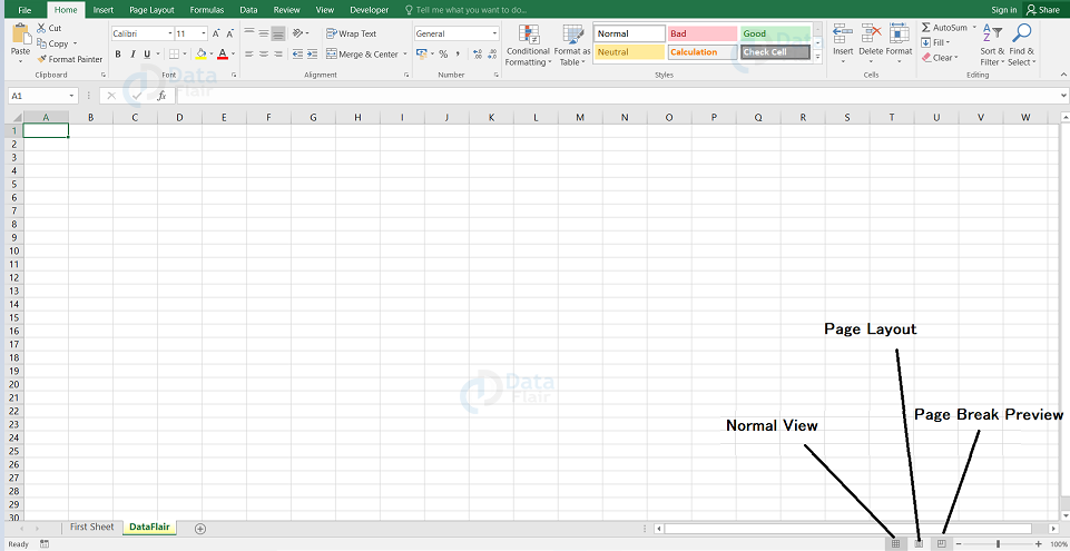
There are a variety of displaying options that change the excel worksheet view. There are Normal view, Page Layout view, and Page Break view available in Excel. These views can be useful in many tasks and this widely helps the user to print the spreadsheet. The user can choose the view of the workbook.
To change the view, choose the required worksheet view from the bottom-right corner of the Excel window.
Entering data in excel:
To enter the data in an excel spreadsheet, double click on the cell and type the data.
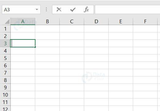
Here, the cell A3 is being selected and once, you enter the data, press enter or you can make use of the arrow keys to navigate from a cell.
Inserting Data in Excel:
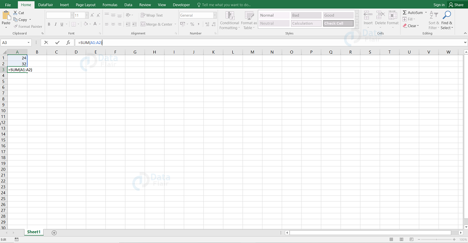
To enter the data in the cell, simply click on the cell and type the data. If it’s a formula, the user has to enter it in the cell or in the formula bar which is available in the top of the cells.
Selecting Data in Excel:
The user can select the data in two ways. The simplest way is to make use of the mouse. Choose the required cell and double click on it.
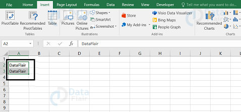
Here, the A2 and A3 cells are being selected.
If in case, the user wants to select a complete section of data then simply place the mouse and drag it down till that last cell you want to select in the sheet. The other method is to use the Go to dialog box.
In order to activate this box, the user can either click on the home tab and choose the Find and Select option or press Ctrl + G from the keyboard. The user will see the dialog box appearing and that box holds an option such as special. Select it and the user will see another dialog box as shown.
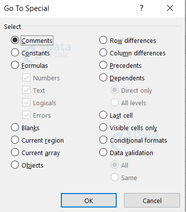
In this box, check the appropriate options that the user wants to select and click on the OK button.
Copy-paste Data in Excel:
Copy and Paste:
If the user wants to Copy and Paste data in Excel, they can follow any of the ways from below:
- Choose the data that the user wants to copy
- Right-click and select Copy the option from the menu.
- Click on the first cell where the data to be positioned and choose the paste option from the menu by right-clicking on that desired cell.
Excel also provides a clipboard that will hold all the data that the user has copied from the sheet. In case, if the user wants to paste any of that data, simply select it from the clipboard and choose the paste option.
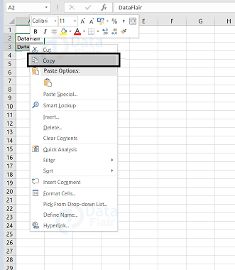
Here, the A2 and A3 cells are being copied.

If D2 is the cell where you wanted to paste the data records, then right click on the cell and choose the paste option.
Note: You can also use ctrl+c to copy the data and ctrl+v to paste the data.
Move the Data:
Excel allows the user to move the data easily to the required location. The user can do in two steps:
Step 1: Select the data and right-click on it.
Step 2: Choose the “Cut” option and click on the first cell where you want the data to be positioned and paste it using the “Paste” option by right-clicking on that desired cell.
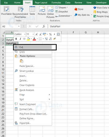
Here, the A2 and A3 cells are being moved to the desired cell.
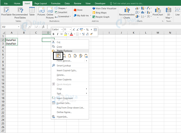
If D8 is the desired cell, then right-click on that cell and choose the paste option. The data will be moved from A2,A3 cell to D8, D9 cell in the spreadsheet.
Delete Data:
To delete any data in the worksheet, the user can use any of the following techniques:
- Select the cell, click on the data and press the Delete button from the keyboard.
- Choose the cell or cells whose data must disappear, right-click on it and choose the Delete option.
- The user can also click on the row number or column header to delete the whole row or column.
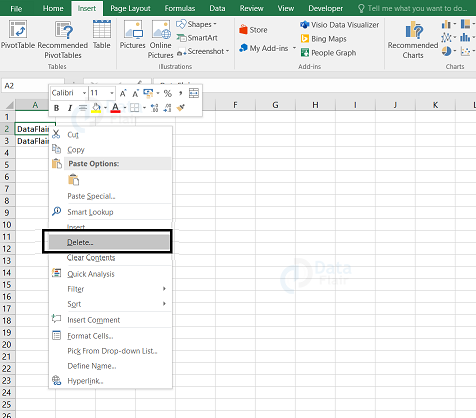
Here, the A2 data record will be deleted from the spreadsheet.
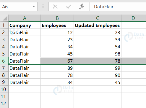
How to delete a row in Excel?
To delete a row, follow the step:
Right-click on the row number and select the delete option.
Note: If you want to delete more than a row, select on the rows, right click on the mouse and choose the delete option.
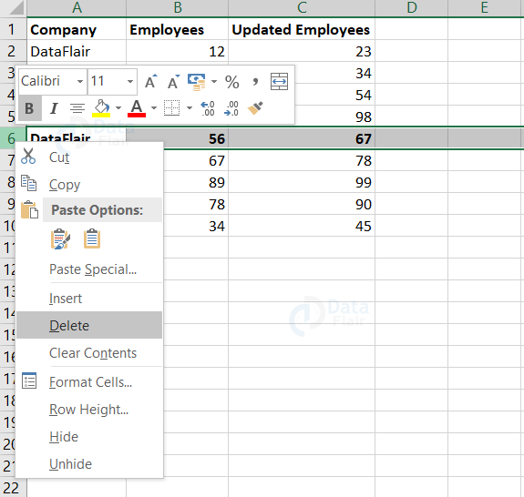
After clicking on the delete option, the 6th row is deleted and the 7th row data values are being shifted to the 6th row cells.
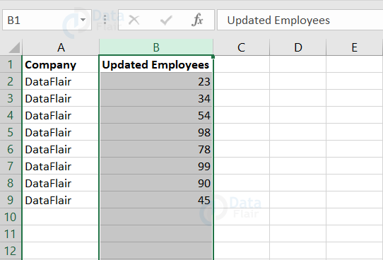
How to Delete a Column in Excel
To delete a column in Excel, follow the step:
Right-click on the column header and select the delete option.
Note: If you want to delete more than a column, select on the columns, right click on the mouse and choose the delete option.
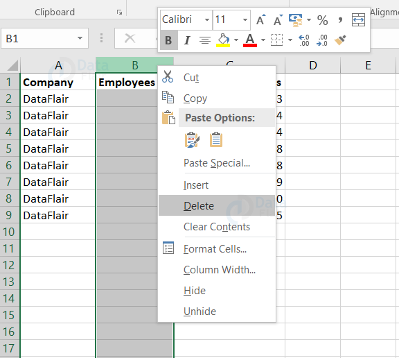
After clicking on the delete option, the B column cells are deleted and the C column cells are being shifted to the B column cells.
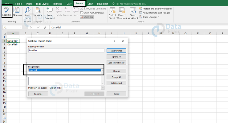
Spell Check in Excel:
To check the spellings of the data, select the data, click on the review tab and choose ‘ABC Spelling’ from the ribbon. Once you click on it, a box appears with the suggestions.
Insert Symbols/Equations in Excel:
You can add symbols and equations in your worksheet. To insert symbols/equations, follow the steps:
1: Select the cell
2: Go to the ‘Insert’ tab
3: Choose either ‘ Symbols’ or ‘Equations’ from the ribbon
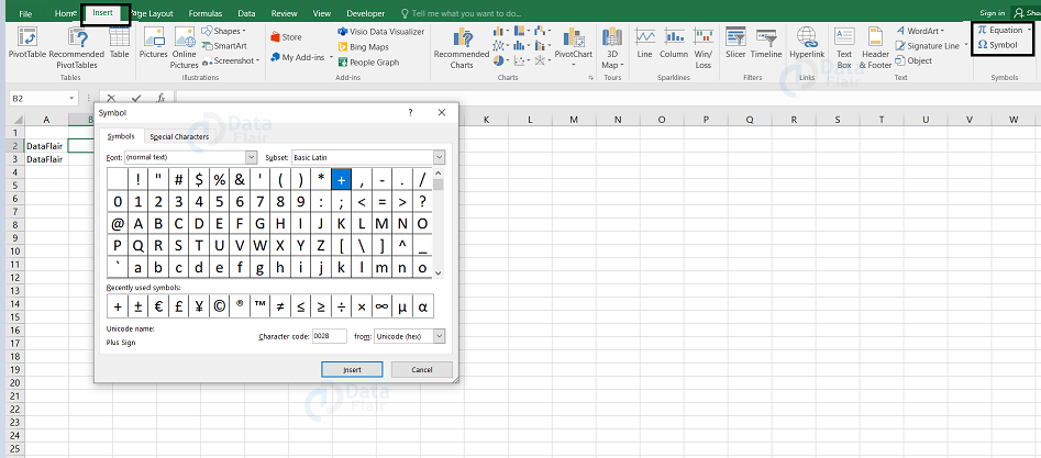
4: Insert the required symbols and click on the ‘Insert’ button.
Other Activities in Excel Sheet:
We can also perform various activities in a worksheet such as:
- Selecting a worksheet
- Inserting a worksheet
- Deleting a worksheet
- Renaming a worksheet
- Moving a worksheet
- Copying a worksheet
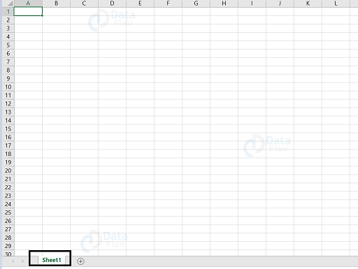
Selecting a worksheet:
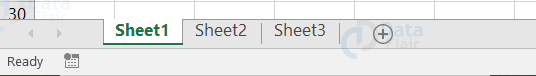
When you open the excel application, it automatically selects the sheet1 worksheet for you. The sheet1 is the default name for the first spreadsheet in your excel and it is viewed in the sheet tab at the bottom of the document.
Inserting a worksheet:
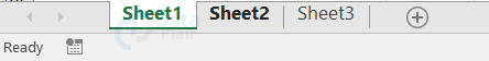
You can work upon more than one worksheet in an excel file. In order to insert a worksheet, click on the ‘+’ symbol in the sheet tab.
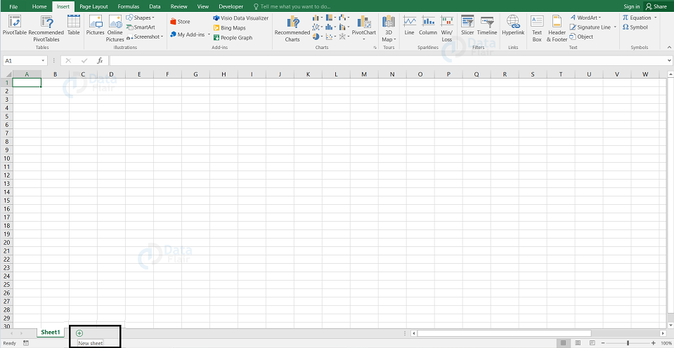
When you click on the ‘+’ symbol, then, a new worksheet will be available in the same file itself.
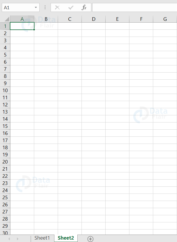
Hope, you observed that ‘sheet2’ is newly formed in the sheet tab at the bottom of the document.
How to hide a worksheet:
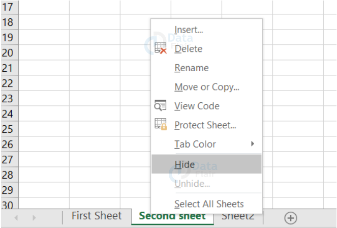
The workbook contains one or more worksheets in it. We can also hide the worksheets if we want to. To hide a specific worksheet, right click on the sheet and choose the hide option.
Unhiding a worksheet:
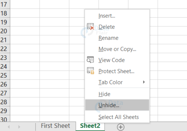
To unhide a worksheet, right-click on any sheet and choose the Unhide option. The hidden worksheets will be visible back again in the sheet tab.
Deleting a worksheet:
You can delete a worksheet, by right-clicking on the sheet tab and choosing the delete option.
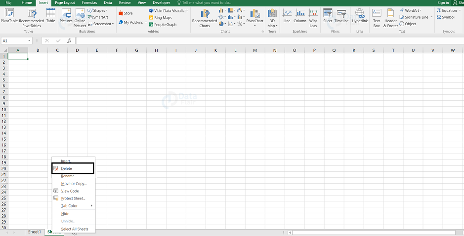
Once you click on the delete option, then that particular sheet gets deleted.
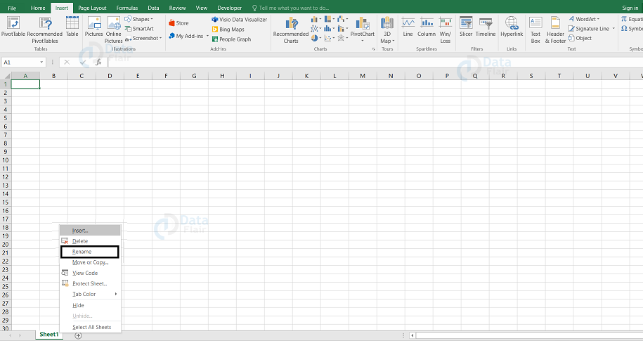
Renaming a Worksheet:
To rename a worksheet, right-click on the sheet and choose the ‘rename’ option.
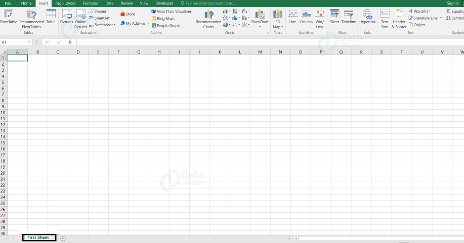
Hope, you observed that the ‘sheet1’ is changed to ‘First Sheet’ in the sheet tab.
Moving a worksheet:
You can also move worksheets by clicking on them and dragging it to the desired position.
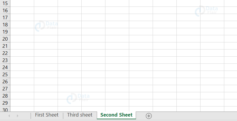
For example, click on the second sheet and drag it in front of the third sheet.
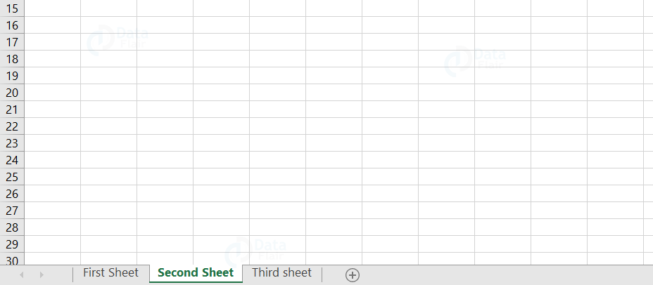
Hope, you observed that the ‘Second sheet’ is before the ‘Third sheet’ now.
Copying a worksheet:
You can also copy the data records of one worksheet to another worksheet. To copy a worksheet, follow the steps:
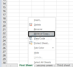
1: Right-click on the worksheet that should be copied.
2: Choose the ‘ Move or Copy ’ option.
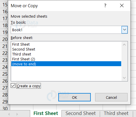
3: Check on the ‘create a copy’ and choose ‘(move to end)’.
4: Press ok
Once you click on it, a new worksheet appears with all the data records from the copied worksheet.
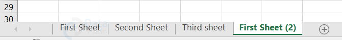
Hope, you can see that a new worksheet is created in the workbook.
Scrolling Across a worksheet:
To scroll a worksheet, you can make use of the scroll bars that are being provided in the spreadsheet.
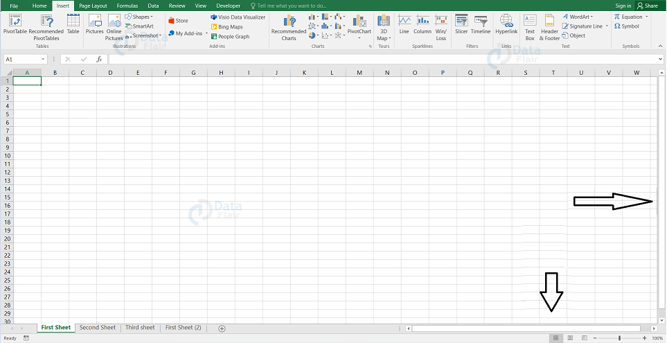
You can use that vertical scroll bar to scroll upwards or downwards and the horizontal scroll bar helps you to navigate to left and right in a worksheet.
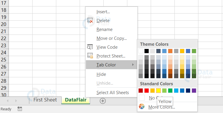
Sheet Tab Color:
You can also highlight the sheet name with a color and in order to highlight your sheet with a color, right click on the sheet name, choose the tab color option and choose the color as per your convenience.
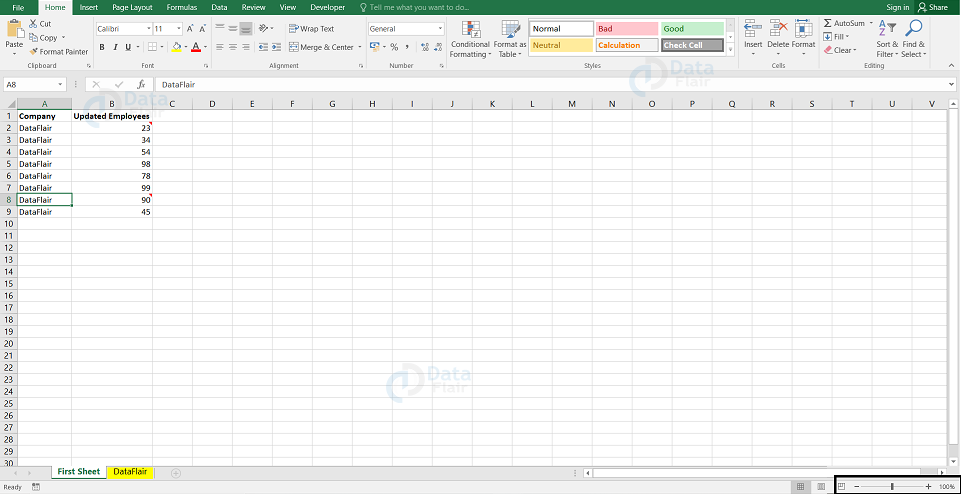
Zoom Slider in Excel
The screen is displayed at 100% in MS Excel by default. The user can change the zooming percentage from 10% to 400 %. Zooming has no effect on the printed output as it does not change the font size.
Zoom slider is present at the right bottom of the workbook.
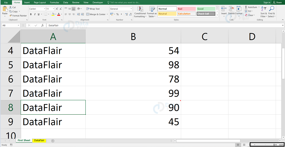
Zoom In
Shift the slider to the right to zoom in the worksheet. The maximum to zoom in is 400% and this changes the view of the worksheet.
Zoom Out
Shift the slider to the left to zoom out the worksheet. The minimum to zoom out is 10% and this changes the view of the worksheet.
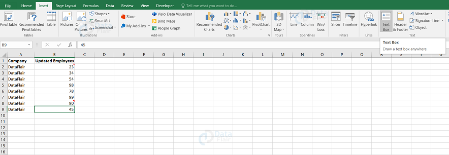
Text Boxes in Excel
Text boxes and cell comments are more similar. They display the text in a rectangular box. The only difference between text boxes and cell comments is that cell comments are visible only when the user clicks on the cell whereas the text box is always visible.
To add a text box, follow the step:
- Click on the insert tab and choose the text box
- Draw the text box in the worksheet or choose a text box.
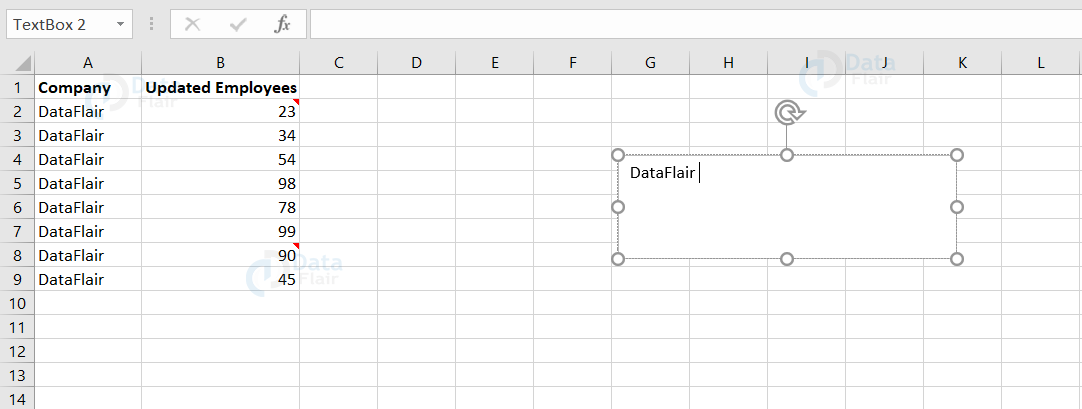
Formatting Text Box in Excel
The user can also format the text box. By formatting, the user can change the font style, size and alignment etc. The important options available in text box formatting are:
- Fill – This option specifies the filling of a text such as No fill, solid fill. The user can also specify the transparency of text box fill.
- Line Colour – This option specifies the line colour and transparency of the line.
- Line Style – This option specifies the width and line style.
- Size – This option specifies the size of the text box.
- Properties – This option specifies the properties of the text box.
- Text Box – This option specifies the text box layout, auto – fit option and internal margins.
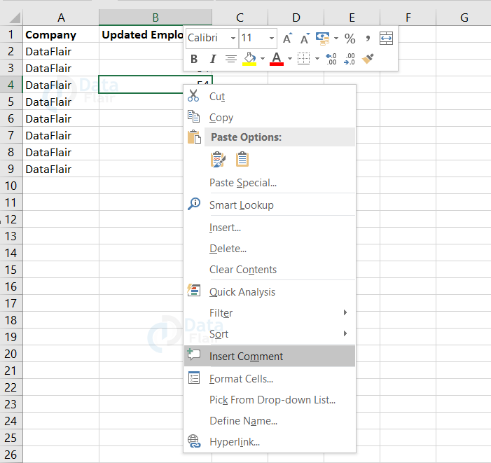
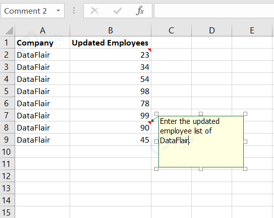
Adding Comment to Excel Worksheet:
The user adds comments to help in understanding the purpose of the cell. This widely helps in having proper documentation.
To add a comment, follow the step:
- Right-click on the cell and choose the ‘Insert Comment’ option.
- Or else, press the Shift + F2.
Note: Initially, the comment box consists of the computer’s username. You can also modify it in the cell comment.
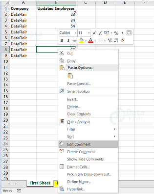
Modifying Comment in Excel:
The user can also modify the comment. To modify the comment, follow the steps:
1: Right-click on the cell on which the comment appears.
2: Choose the edit comment from the list of options available.
3: Modify the comment as per the requirement.
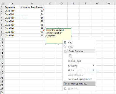
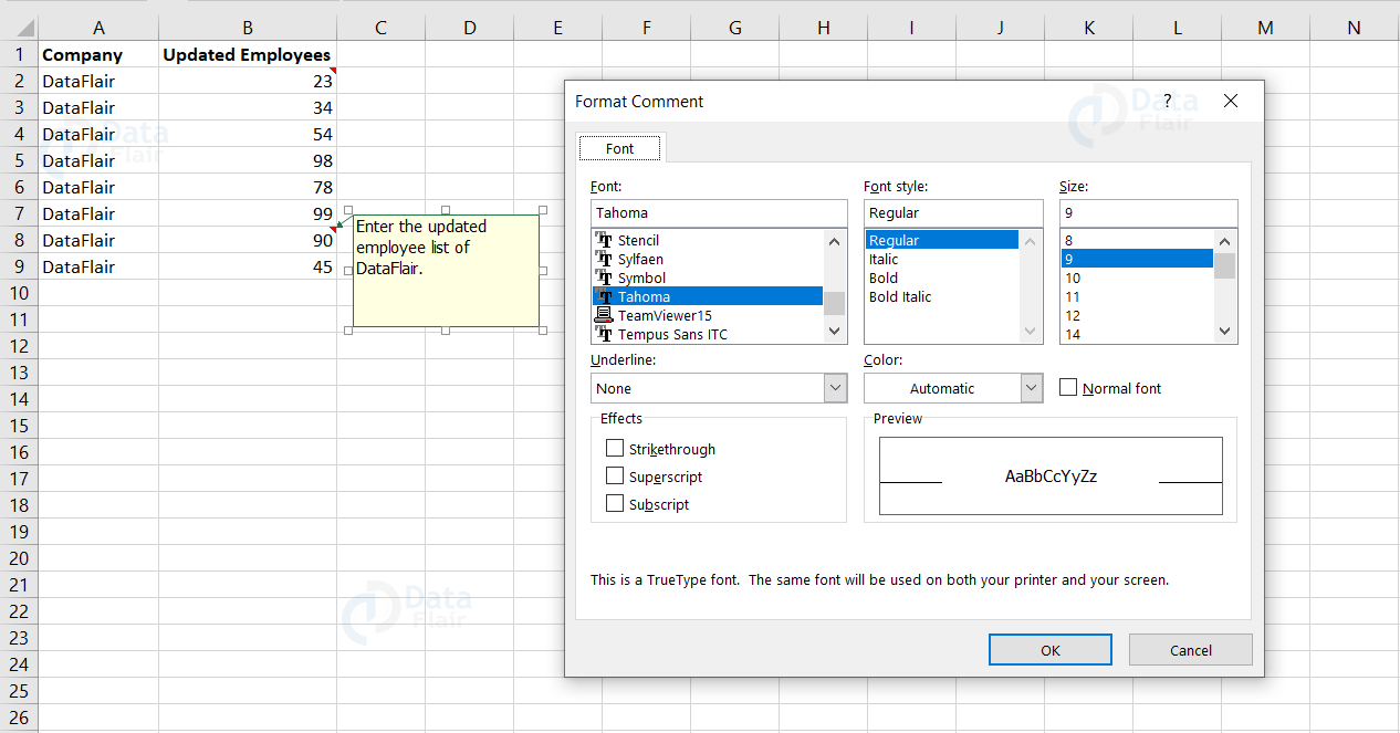
Formatting the Comment in Excel:
There are also formatting options available for comments. Using formatting, the user can change the color, size and font style of the comment.
To format a comment, follow the steps:
- Right-click on the cell
- Choose Edit comment from the options available.
- Select the comment and right-click on it
- Choose format comment from the options.
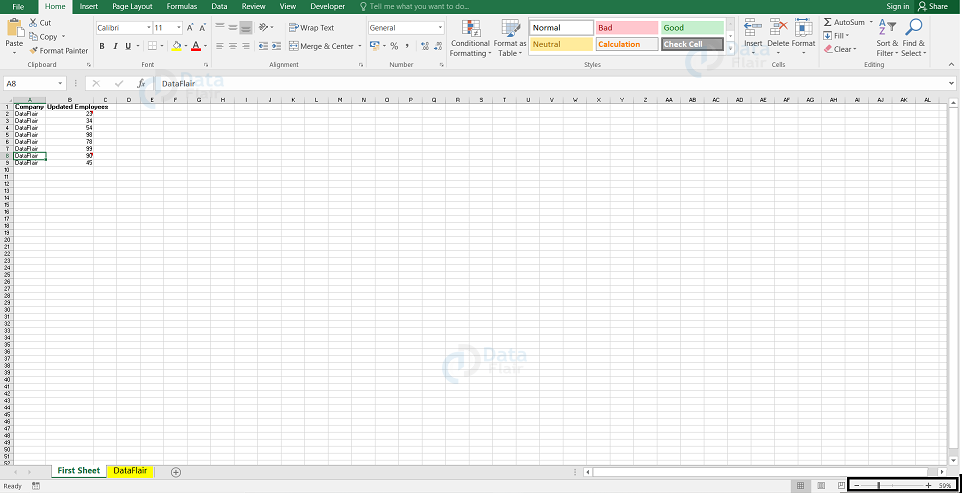
Changing the default count of sheet numbers:
You can also change the number of worksheets that appear, when you open a workbook. In default, the sheet number is 1 and in order to change the count of sheet number, click on the file tab, choose option, go to general and change in “include this many sheets” label.
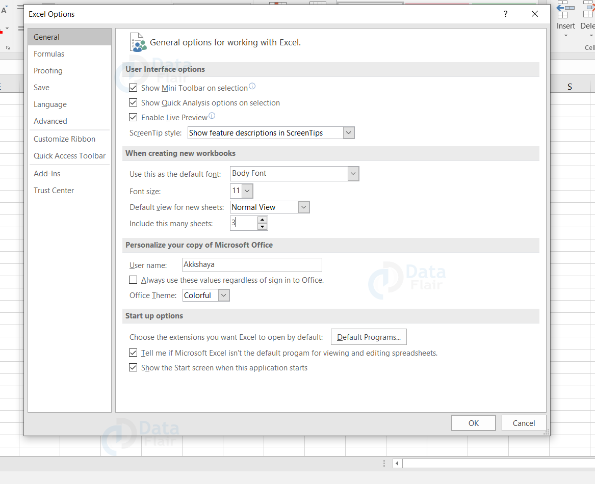
Here, we have changed the number of sheets to 3.
Undo Changes in Excel sheet
Using the Undo command, the user can reverse the actions in MS Excel. To undo changes, follow the step:
- Click on the undo icon from the quick access toolbar.
- Or else press Ctrl+Z
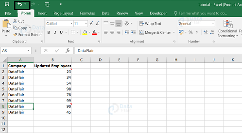
Note: The user can reverse nearly 100 past actions that are performed by executing undo more than once. The list of the actions appears when the user clicks on the arrow button. Click an item from the list to undo that particular action.
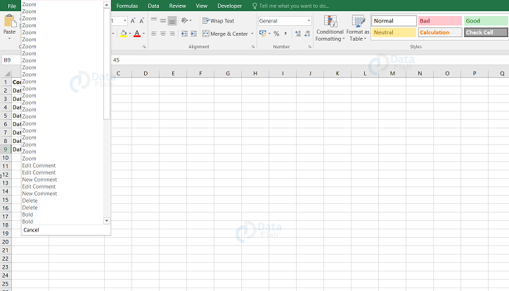
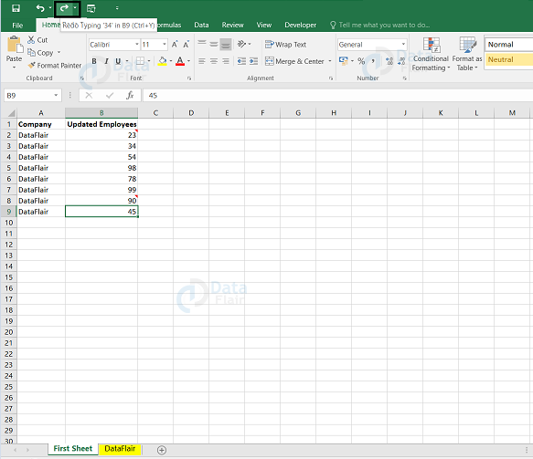
Redo Changes in Excel Sheet
The user can also reverse back the action by clicking on the Redo icon.
To Redo changes, follow the steps:
- Click on the redo icon from the quick access toolbar.
- Or else press Ctrl + Y
Merging the cells in Excel sheet:
You can merge or unmerge the cells in a spreadsheet. If you merge a cell, it acts like a single cell.
To merge a cell, select the cells and choose the merge & center option from the home tab.
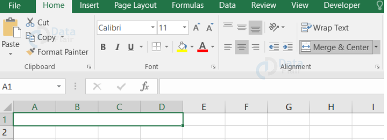
Here, the A1, B1, C1, D1 cells are being merged and hence they will behave like a single cell.
Shrink/ Wrap
Shrink and wrap text options are hugely helpful to align and set the size of the text.
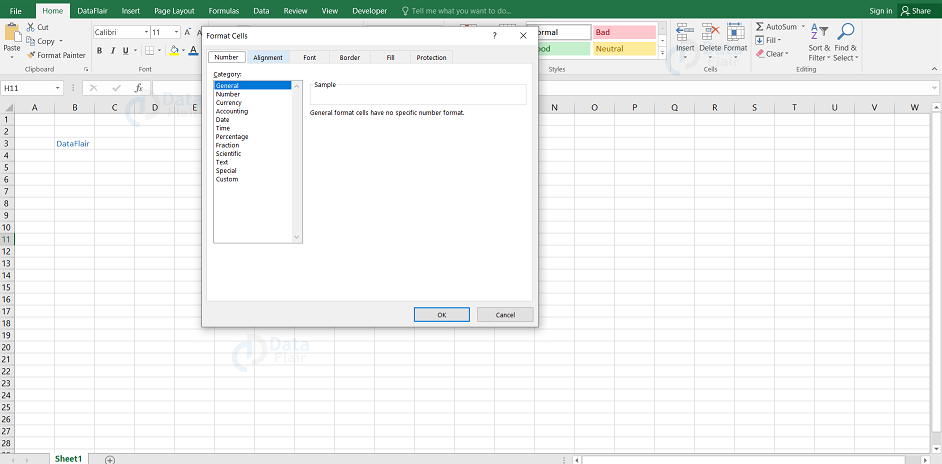
Cell type
The data in the cell can be of any type and format. Some of the cell types are listed below
| Type | Description |
| General | Allows any type of data. |
| Number | Displays in the format of numbers. |
| Currency | Displays in the format of currency. |
| Accounting | Account purpose data are entered in accounting purpose. |
| Date | Displays in the format of date. |
| Time | Displays in the time format. |
| Percentage | Displays the values in percentage. |
| Fraction | Displays in the format of fraction. |
| Scientific | Displays in the exponential form. |
| Text | This format is used when the data is in text format. |
| Special | Special formats are used in case of entering telephone numbers etc |
| Custom | The format can be customized as per the user convenience |
Borders in excel
You can add borders and shades to a cell in the spreadsheet. To add borders, select the cell, right click on it, choose the format cells option and then click on the type of border that you would like to add to that cell. You can also change the thickness, style, color etc.
Decorating and formatting the data in Excel
You can also decorate and format the data in an excel spreadsheet. To decorate and format, right click on the cell, choose format cells option and click on the font tab in the dialog box window. After making the required changes in the font type, style and size, click on the ok button.
Excel Context Help:
Excel context help is a feature in excel which provides appropriate information about the Excel commands in order to make the user know about its usage and working.
Editing the Excel Worksheets:
The user can also edit the data that they enter in the worksheet. The user can enter in any form such as text, numeric or formulae.
Formatting MS Excel Worksheets:
Sheet Options:
There are a number of options available for taking the printouts. The user can select an option from it and print the sheet in various ways. To click on the sheet options, choose the page layout group from the home tab, open the page setup. You can see a various number of sheet options and they are listed below:
| Option | Description |
| Print Area | The user can set the print area. |
| Print Titles | It allows the user to set the row and column titles at the top. |
| Gridlines | The user can add the gridlines to the printout. |
| Black and White | The user can take the print out in black and white. |
| Draft Quality | It allows the user to print the sheet using the printer’s draft quality. |
| Row and Column Headings | It allows the user to print the row and column headings. |
| Down, then over | It prints the down pages first and it is followed by the right pages. |
| Over, then down | It prints the right pages first and it is followed by the down pages. |
Excel Margins and Page Orientation:
Margins:
The margins are the unprinted regions on the top-down and left-right sides. Each and every MS Excel page has borders and if the user selects some border for a page, then that border appears to those particular pages.
Note: The user can’t have different margins for each page. The user can add margins in the following ways:
- Select the page setup from the page layout tab and then the user can click on the margins drop-down list.
- The user can also add Margins while printing the excel page. In order to perform that, click on the File tab and choose Print. Here, the user will be able to see a dropdown list having all the Margin options that are available in Excel.
Page orientation
Page orientations are of two types and they are portrait and landscape. The page orientation helps the user to select the format in which the sheet is printed. The portrait orientation prints the page taller and the landscape orientation prints the sheet wider. To select a type of page orientation, choose the drop-down list from the page setup group and click on the appropriate orientation. The user can change the page orientation while printing the excel sheet.
Excel Headers and Footers:
Headers and footers provide some information at the top and bottom of the page. The header and the footer are not available in a new workbook. In order to add the header and footer, the user can open the page setup window and open the header/footer pane. The user will have a number of options to customize the headers and footers.
If the user wants to preview the header and footer that are added, click on the print preview option and the user can see the changes.
Page Breaks:
MS-Excel allows the user to control what they want to print and what they want to omit. Using page breaks, the user can control the page print such as restrain from printing the first row of a table at the end of a page or printing the header of a new page at the end of the previous page. The page breaks will allow the user to print the sheet in order to the preferences. The user can have both horizontal and vertical page breaks. Select the row or column to include the page break and then go to page setup, choose the options from insert page break.
Horizontal Page Break:
To add a horizontal page break, select the row where the user wants to introduce the break from.
Vertical Page Break:
To add a vertical page break, choose the column where the user wants the page to break from.
Removing Page Breaks
- The user can remove a page break that is added. To do so, move the pointer to the first row and then choose the page layout, choose the page setup, select breaks, and remove page breaks.
- The user can remove all the manual page breaks. To do so, choose the page layout, click on the page setup, select break options and reset all page breaks options.
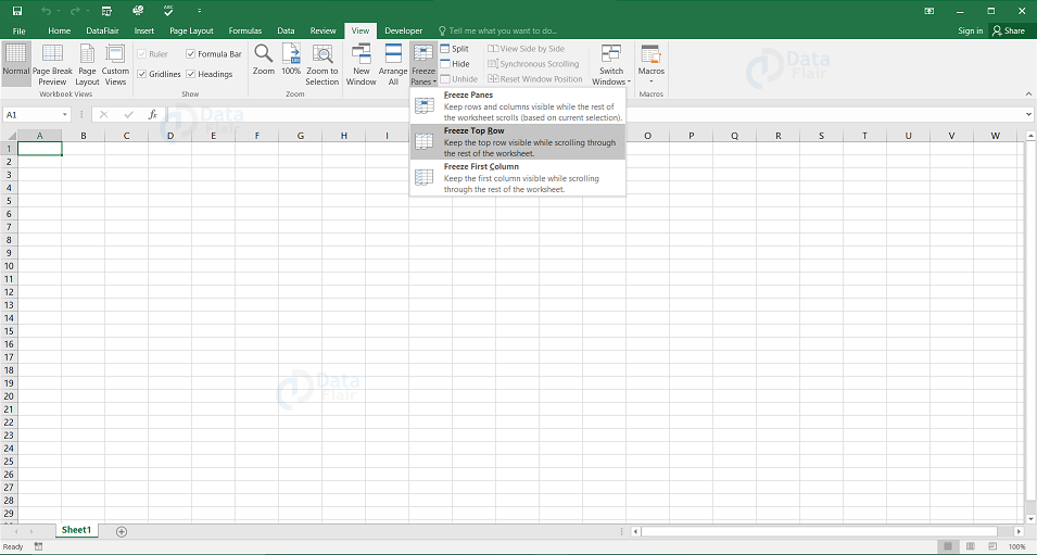
Excel Freezing Panes:
The freezing panes enable the user to see the row and column headings even if the user keeps scrolling down the page. In order to freeze panes, the user has to:
1. Choose the rows and columns that have to be freezed.
2. Go to the view tab and choose the freeze pane group.
3. There will be three options to freeze rows and columns.
Unfreeze Panes
To unfreeze the panes, go to the View Tab and select unfreeze panes.
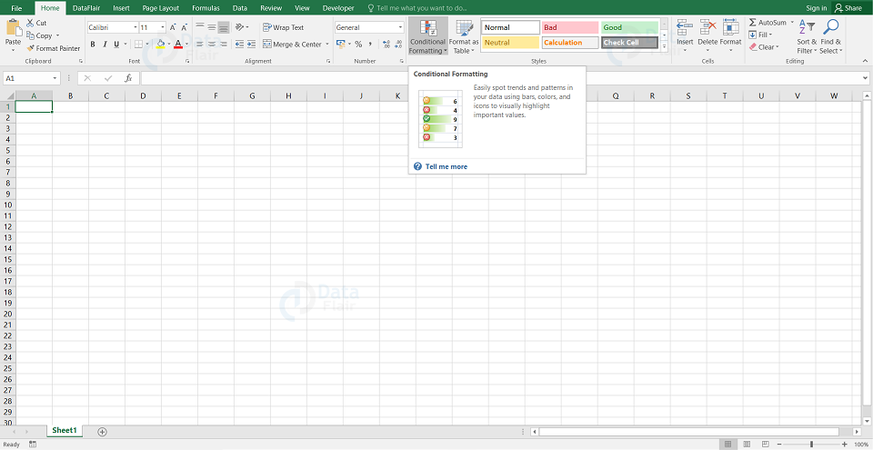
Excel Worksheet Conditional Formatting:
Conditional Formatting allows the user to selectively format a section to hold values within some specified range. The values outside the ranges will be formatted automatically and there are features which has number of options available which are listed below:
| Option | Description |
| Highlight Cells Rules | It opens another list that defines the selected cells containing values, text or dates that are greater than, equal to, less than some specified value. |
| Top/ Bottom Rules | It highlights the top or bottom values, percentages and averages. |
| Data Bars | It opens up a palette with different colored data bars. |
| Color Scales | It opens up a color palette with two and three colored scales. |
| Icon Sets | It contains different sets of icons in it. |
| New Rule | It opens up a new formatting rule dialog box for custom conditional formatting from it. |
| Clear Rules | It allows the user to remove the conditional formatting rules. |
| Manage Rules | It allows the conditional formatting Rules manager dialog box to open up from where the user can add, delete or format rules according to their preferences. |
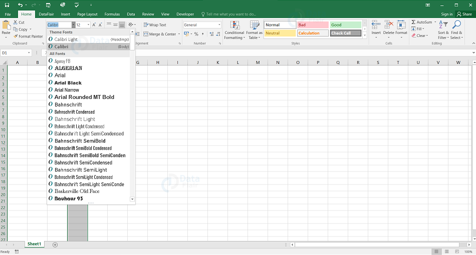
Setting Font from Home
The user can set the font of the selected text by clicking on the Font group from the home tab and then select the font.
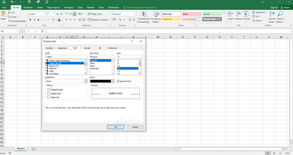
Setting Font From Format Cell Dialogue
- The user can also set the font from the format cell dialogue box by right clicking on the cell, choose the format cells option and then the font tab.
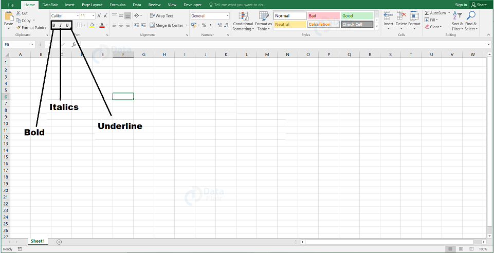
Excel Worksheet Text Decoration
There are various options available in the Home tab of the ribbon and they are:
- Bold − The user can choose this option, if they want the text to appear in bold.
- Italic − The user can choose this option, if they want the text to appear in italics.
- Underline − The user can choose this option, if they want the text to be underlined.
- Double Underline − The user can choose this option, if they want the text to be double underlined.
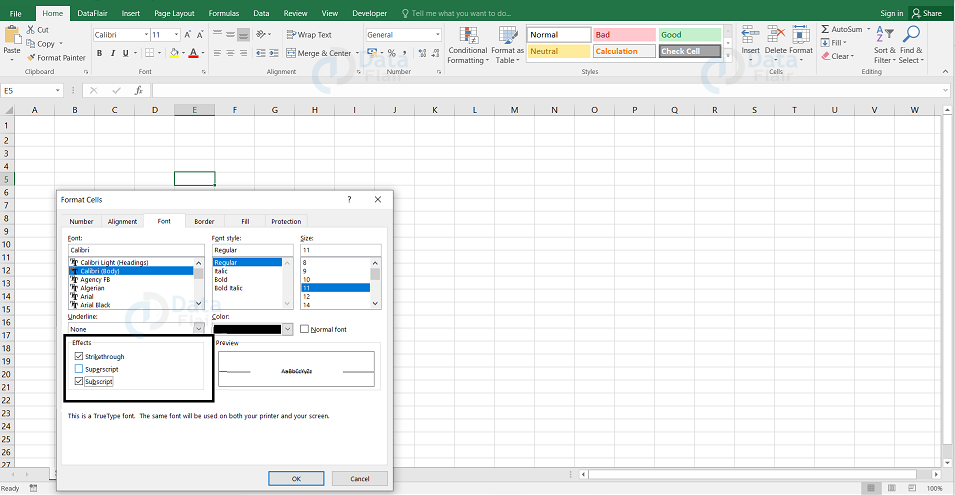
More Text Decoration Options
There are more options available for text-decoration and the user can access it by clicking on the formatting cells from the font tab and choosing the effects as required. The effects available are listed below:
- Strike-through − Strikethrough is an option that strikes the text in the center vertically.
- Superscript − Superscript is an option that makes the content appear as a superscript.
- Subscript − Subscript is an option that makes the content appear as a subscript.
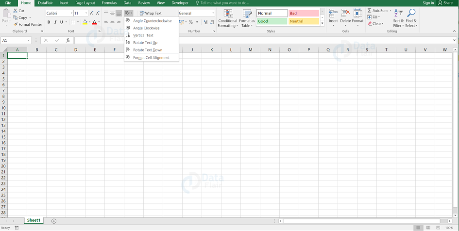
Rotating Cell from Home Tab
There are options available like angle counter-clockwise, angle clockwise etc and the user can reach out to these options through clicking on the orientation under the home tab.
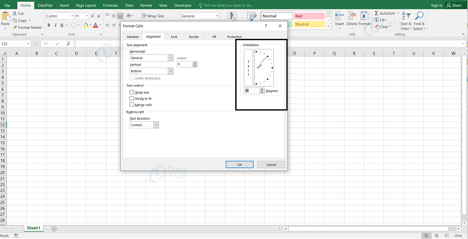
Rotating Cell from Formatting Cell
To rotate the cell from formatting cell options, right-click on the cell, choose format cells, click on the alignment, and set the degree for rotation.
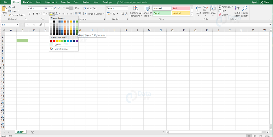
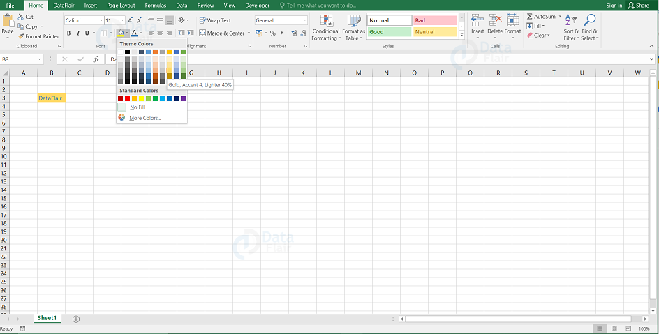
Changing Background Color in Excel
The user can change the background color as per the requirement. To change the background color, go to the font group under the home tab and select the background color. In MS Excel, the background color of the cell is white by default.
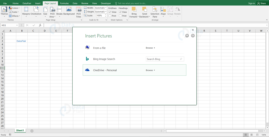
Background Image
The user cannot have a background image on the printouts. The user would have already known about the background command. This background command displays a dialogue box that lets the user select an image to display as a background. The background images on a worksheet will never be printed.
Alternatives to place Background
- The user can insert a shape, WordArt, or a picture on the worksheet, and then they can also adjust its transparency.
- The user can also insert an object in a page header or footer.
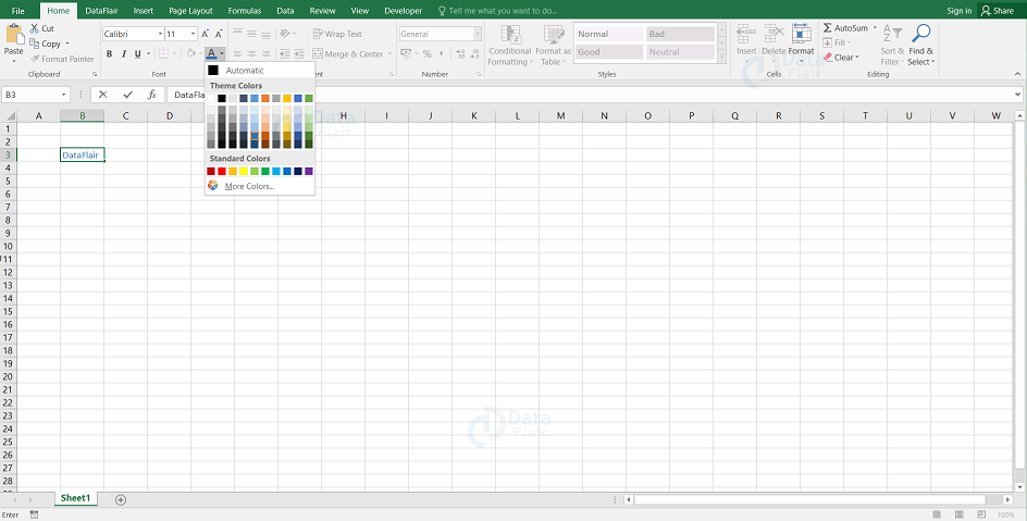
Changing Foreground Color in Excel
The user can change the foreground color as per the requirement. To change the foreground color, go to the font group under the home tab and select the foreground color. In MS Excel, the foreground color or the text color is black by default.
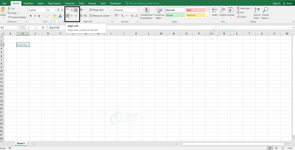
Change Alignment from Home Tab
The user can change the Horizontal and vertical alignment of the cell in Excel Worksheet. To change the alignment, go to the alignment group under the home tab and then select the alignment type. In Excel, the numbers in the cell aligns to the right and the text to the left by default.
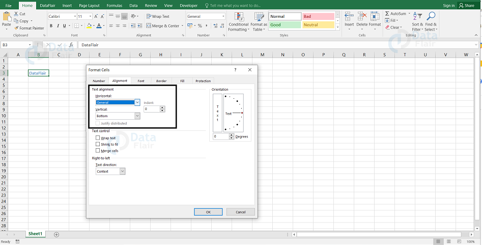
Change Alignment from Format Cells
To change the alignment of the cell from formatting cell options, right-click on the cell, choose format cells, click on the alignment and choose the options from the vertical alignment and horizontal alignment options.
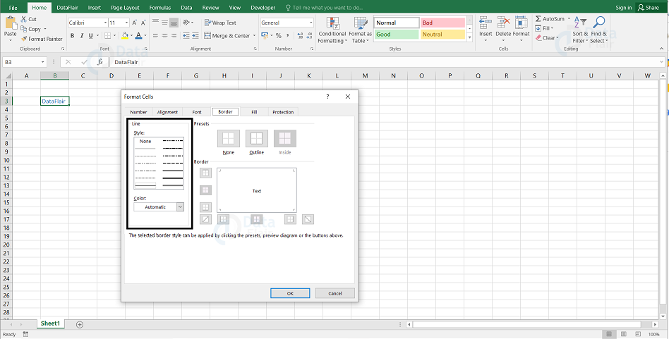
Apply Borders in Excel
The user can apply borders to the cells in MS-Excel Worksheet. To apply a border, follow the steps:
- Select the range of cells or a particular cell.
- Right click on it and choose the format cells.
- Go to the border tab and select the border style.
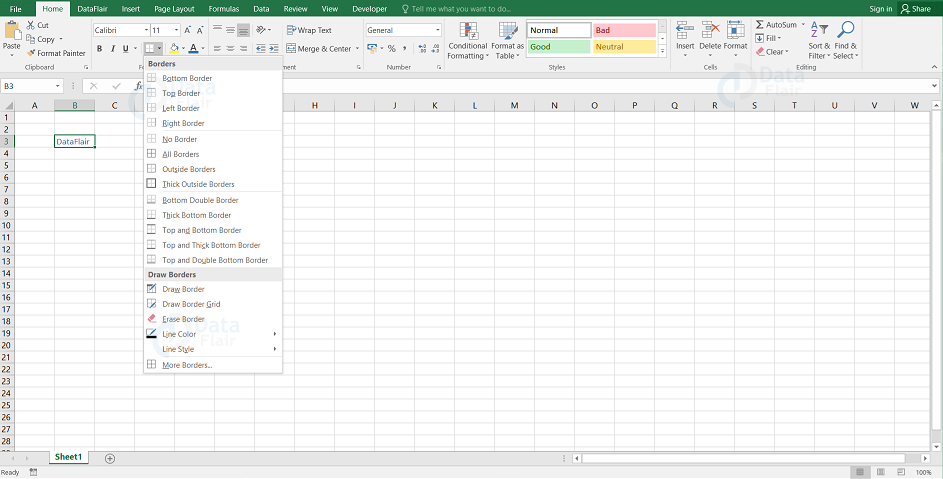
The user can also apply borders to the cells from the home tab also. To do so, click on the apply border options in the font group under home tab.
Apply Shading in Excel
The user can apply shading to the cells from the home tab itself. To do so, click on the color options from the font group under home tab.
Formatting Cells in Excel Worksheet
In MS Excel, the user can apply formatting to the cell or range of cells by right clicking on it and choosing the format cells. The user can select the tab from various tabs available.
Things to Remember
- When we open an excel workbook, we get three worksheets by default.
- The shortcut key to insert a new worksheet is Shift + F11.
- The shortcut key to delete a worksheet is Alt + E + L.
Summary:
- Each worksheet consists of 1048576 rows and 16384 columns.
- It is one of the easy tools where you can enter any amount of data.
- It serves the data in a tabular form and it also allows the user to organize the information.
We work very hard to provide you quality material
Could you take 15 seconds and share your happy experience on Google


