MS Excel Interview Questions

Following are the most important Excel interview questions that an interviewer might ask. These questions and answers would widely help the candidate to prepare for the interview.

MS Excel Interview Questions for Beginners

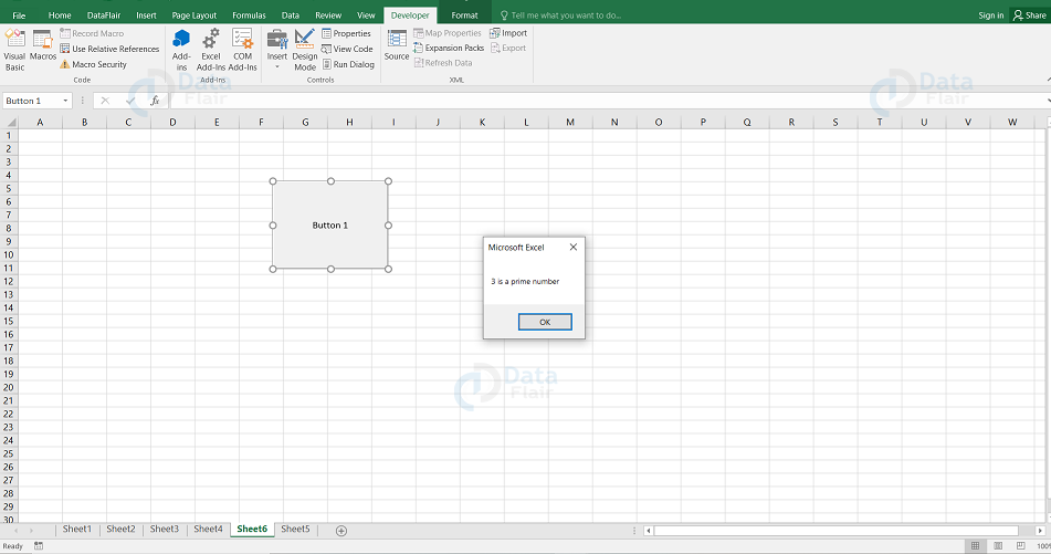
1.Write a dynamic VBA program to check if a number is a prime number ?

Sub Button1_Click()
Dim div As Integer, num As Integer, i As Integer
div = 0
num = InputBox("Enter a number")
For i = 1 To num
If num Mod i = 0 Then
    div = div + 1
End If
Next i
If div = 2 Then
    MsgBox num & " is a prime number "
Else
    MsgBox num & " is not a prime number"
End If
End Sub

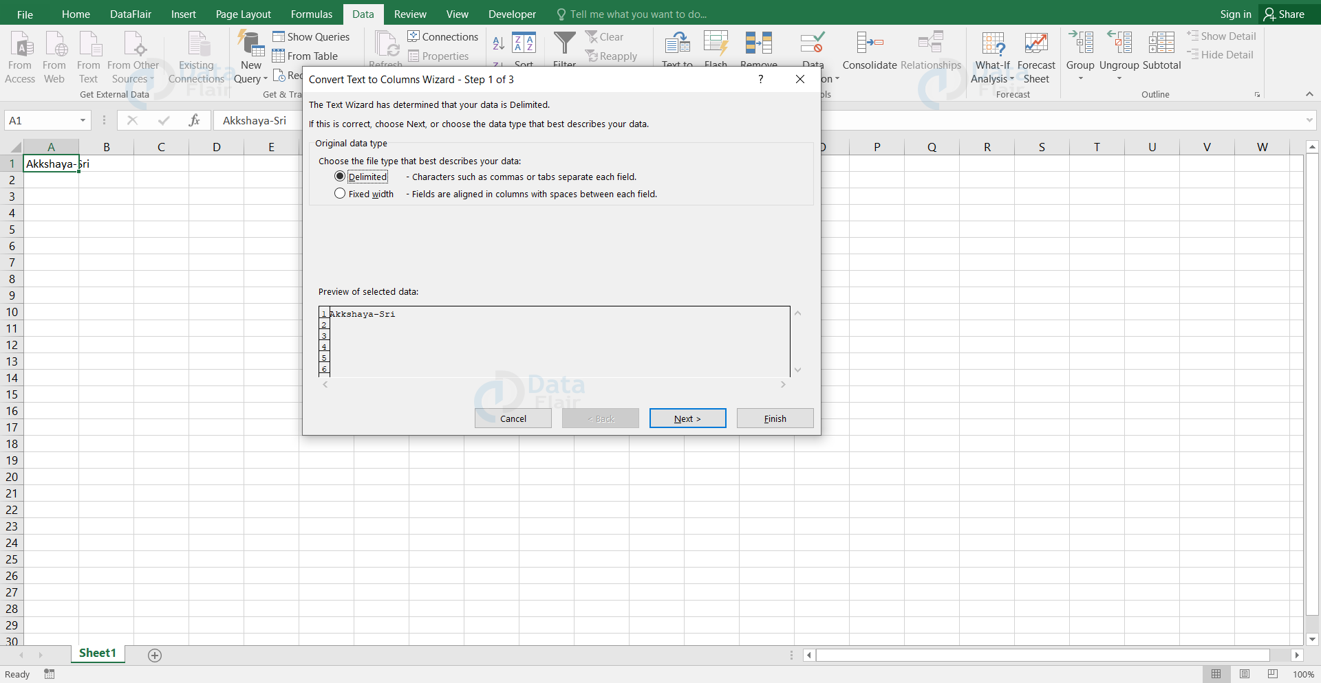
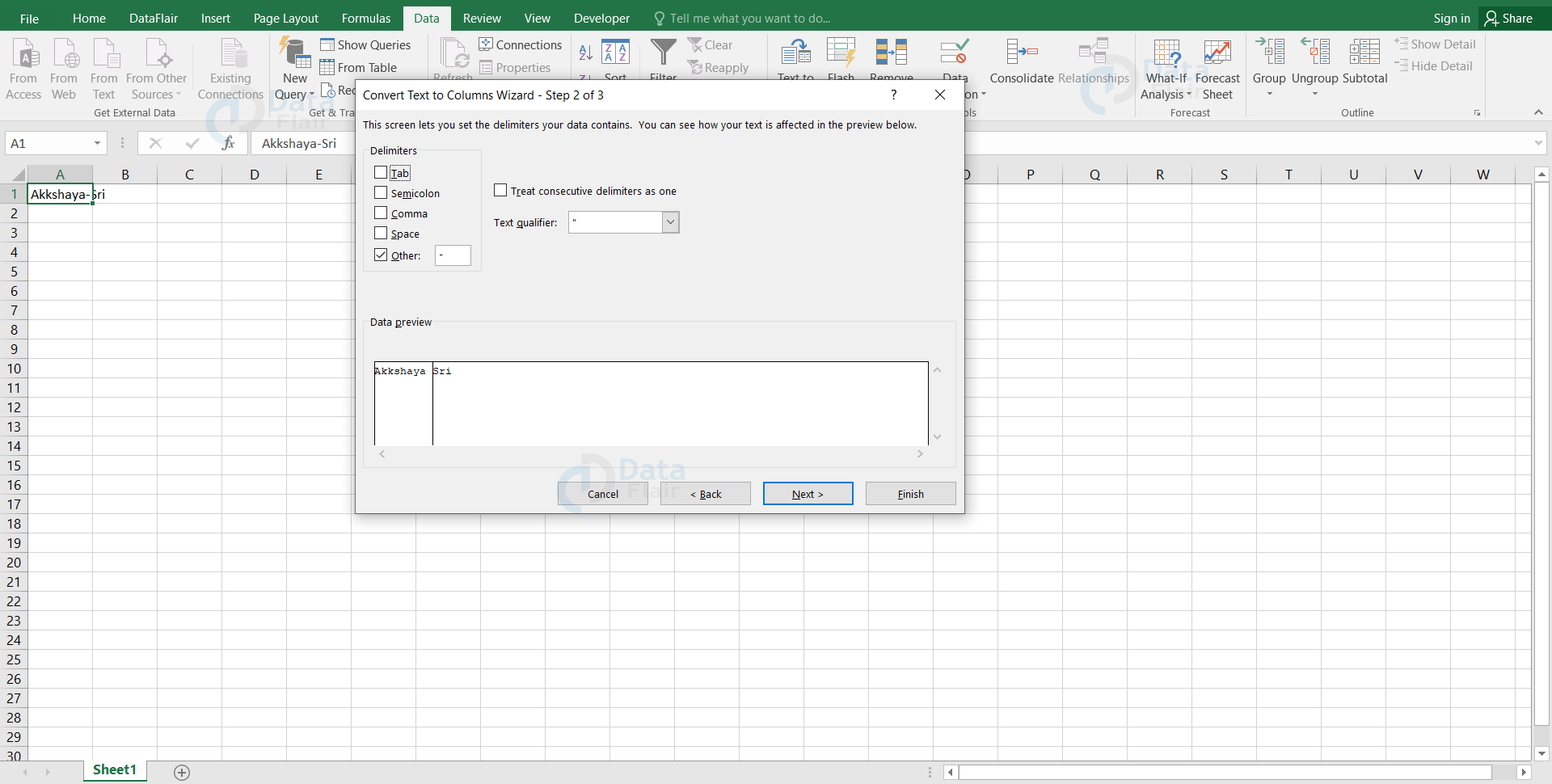
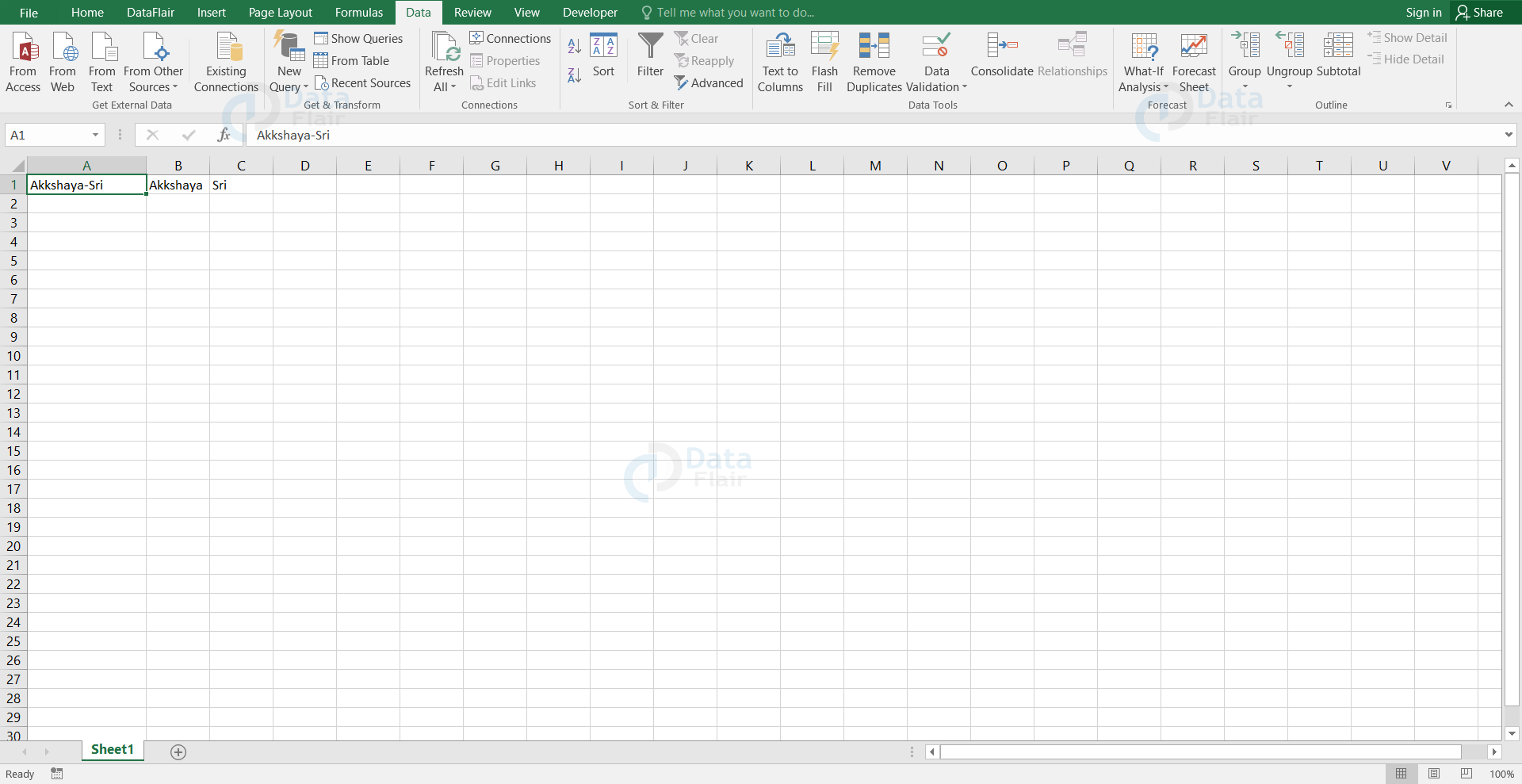
2. Are there any possibilities to split column data?

Yes, we can split the column data into two or more columns. In order to do that click on the cell that you want to split, go to the Text to Columns option under the data tab. After that choose the delimiter options as required. Finally select the column data format and choose the destination to display the split. The final output will appear as a result, separated into multiple columns.

3. What are the alternative ways to perform calculations other than writing the calculations in a cell?

The alternative ways to perform calculations are:

• AutoSum Function – In autosum function, the calculation is performed automatically after the user selects the cells on which the calculation has to be done.
• Insert Function – The insert function pops up with a dialog box where we can type the operation name and find it. After choosing the function, we can perform it on the cells in the worksheet.
• Formulae from the group – There are various groups such as Logical, Math & Trig etc in Excel. We can pick a formula from the related group and work with it.

4. How to set up the input message in MS-Excel?

Setting up the Input message:

a. Select the cell and click on the data validation.

b. Go to the input message tab in the box.

c. Fill the title and message as per the requirement and convenience.

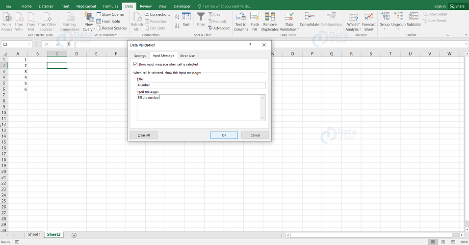
d. Then, press the OK button.

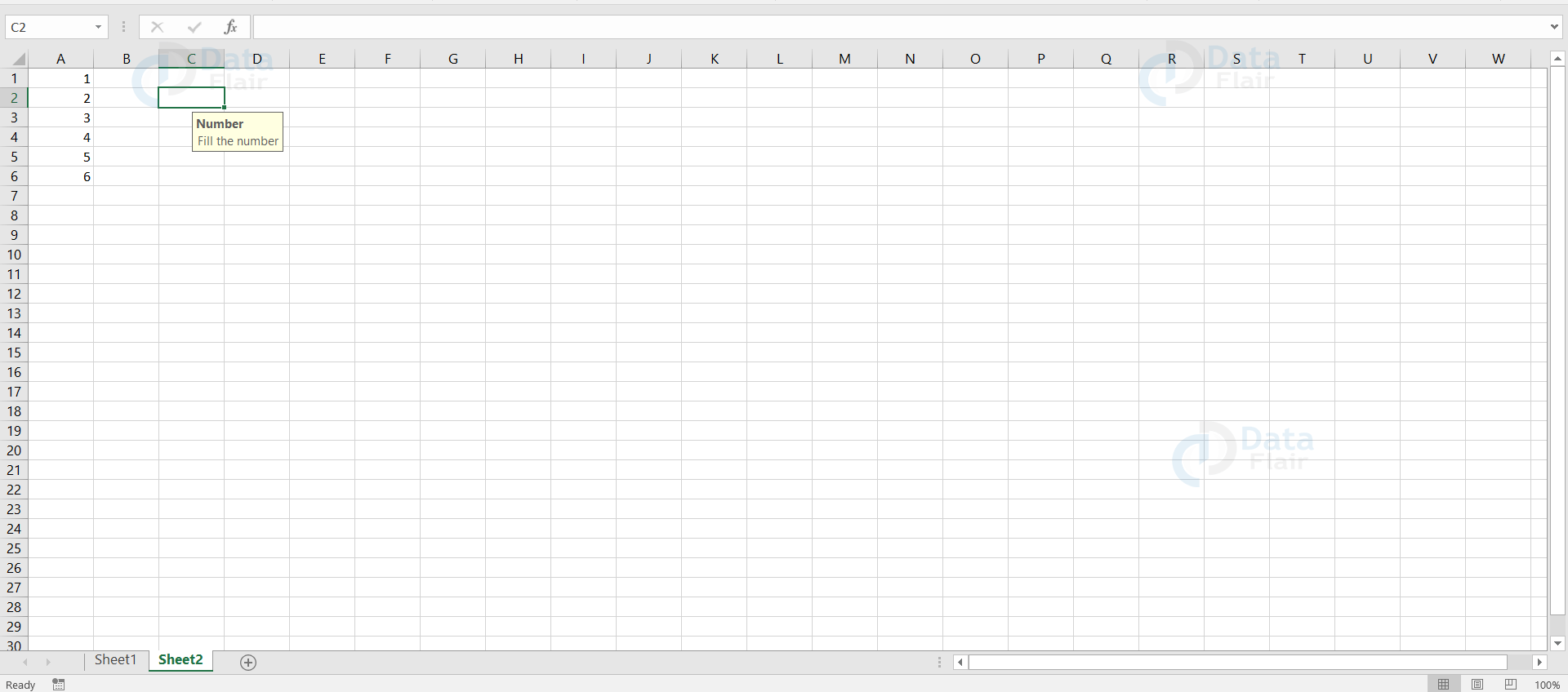
Finally, when you place the cursor on the data validation applied cell, the message will appear in a box as information.

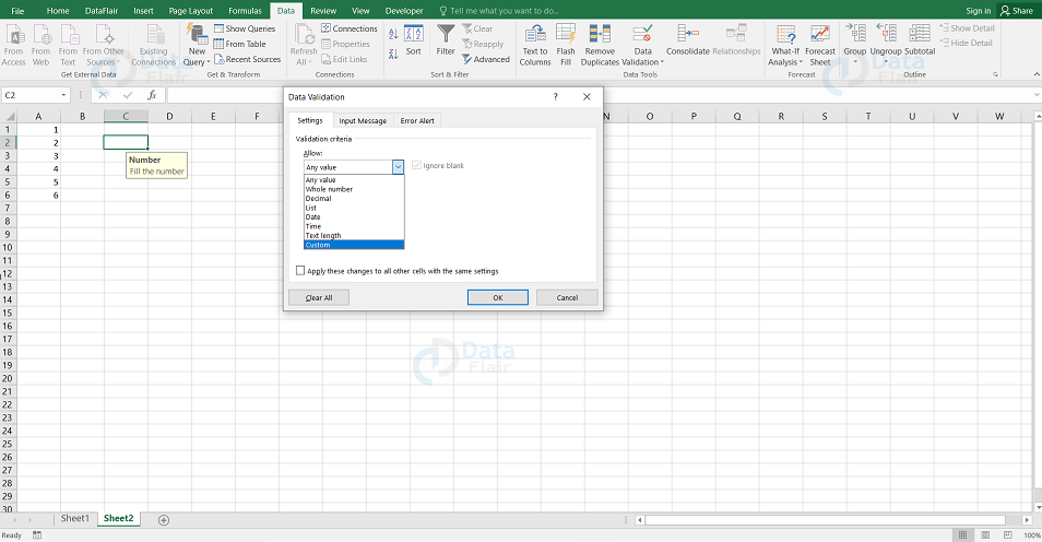
5. How to set up the custom data validation?

Custom Data Validation:
The user can set up the formula as per the requirement and this is known as custom data validation. To set up the custom data validation, click on the data validation option from the drop down under the data tab. Pick the custom as criteria. A window pane appears with the data asking for the formula, type the formula and press the ok button.

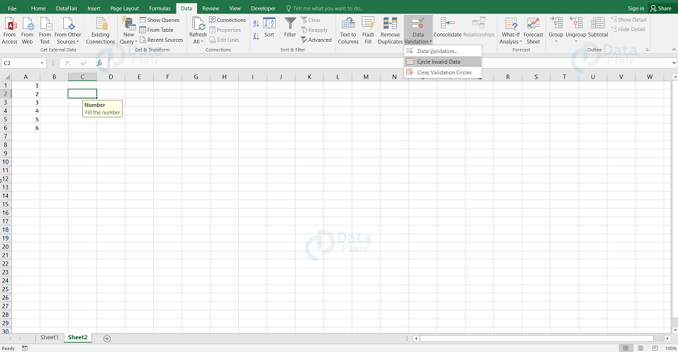
6. Can we circle the invalid data after applying data validation?

To circle the invalid data, first enter the dataset, and then after entering the dataset apply the data validation as per the requirement after that click on the data tab and choose the circle invalid data from the ribbon.

7. Data validation function is one of the best and most effective functions available in excel but there is also a situation where it does not perform its action. Could you tell when it goes ineffective?

Data validation helps the user in setting the rule for the cells in the spreadsheet, not just that it also helps in controlling the value that is being entered in the cell. But there is a scenario where data validation does not apply and that is when the data are replaced on the existing data validated cells and the validation will not be applied if the cells are copied and pasted.

8. What do you know about the wildcards and are they available in excel?

Yes,wildcards are available in excel and the wildcards in excel works only on the text data in the sheet. Excel has three main wildcards and they are “ *, ?, ~” .

Asterisk(*): This symbol refers to any number of characters.

Question Mark(?): This symbol refers to one single character in the sheet.

Tilde(~): This symbol helps in identifying a wildcard character such as “ *, ?, ~” in the text.

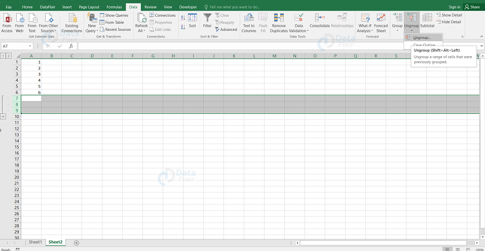
9. What are the steps to ungroup the dataset in Excel?

To ungroup the dataset in excel click on the ungroup option under the data tab and from there we can choose either its row or column.

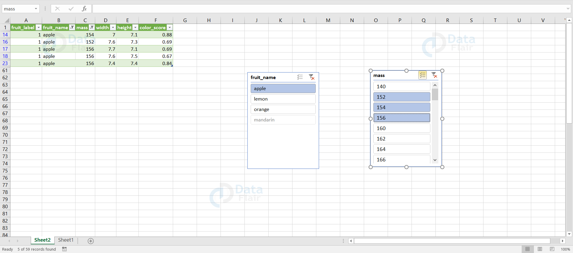
10. How does a Slicer work in Excel?

We use slicers to filter the data in a pivot table. In order to create a slicer, we have to click on the Design tab, and select Insert Slicer. Then, choose the list of fields for which we want to create slicers.

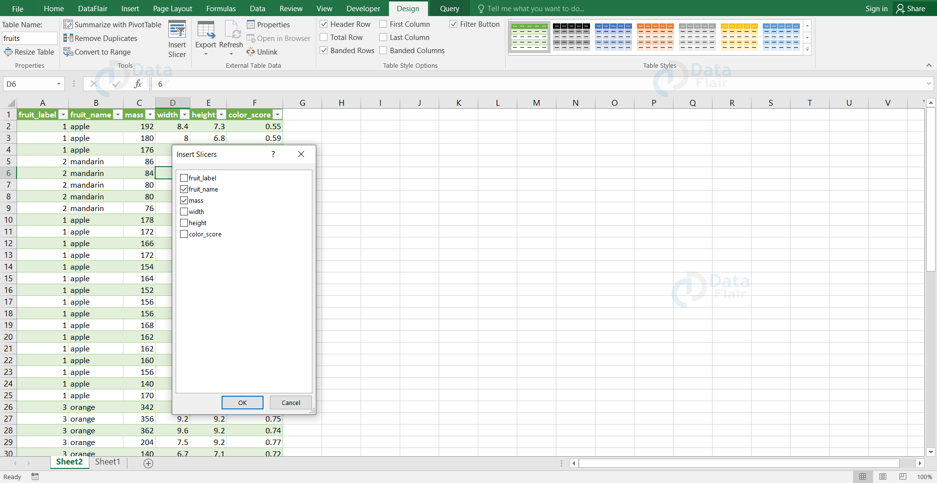
In the below example, we have chosen two labels for the slicers. Hence two slicers appear to filter the pivot table.

Intermediate Excel interview Questions and Answers

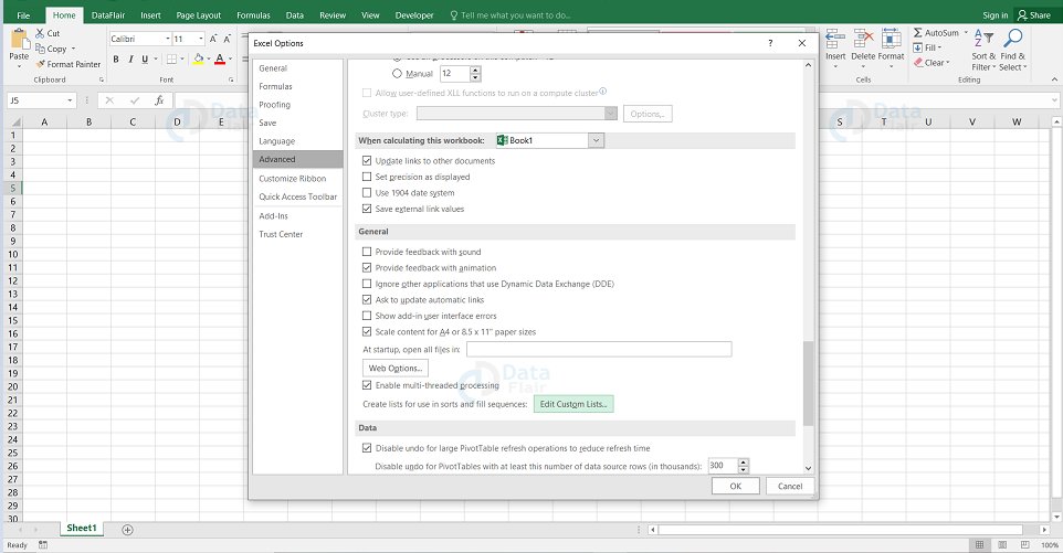
11. What are the steps to customise the auto fill list?

The steps to follow are-

1- To customise autofill, click on the options under the file tab and select the advanced options.

2- Under the heading of general, go to edit the custom list option and a box appears, where we can enter the new list.

3- After updating the list, click on the add button, then the list will be updated in the custom list and it can be accessed in the sheet from then on.

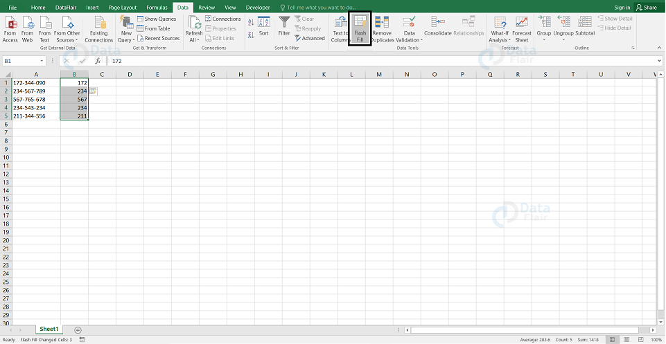
12. What do you know about flash fill and how is it helpful in MS-Excel?

The main use of flash fill is, it helps in filling out the data automatically. If the pattern of the data is analysed then the preview will be shown in a box. It also merges the cell values and auto fills the other cells and it can also separate a value from a cell. In the below example, we can see how flash fill performs its activity.

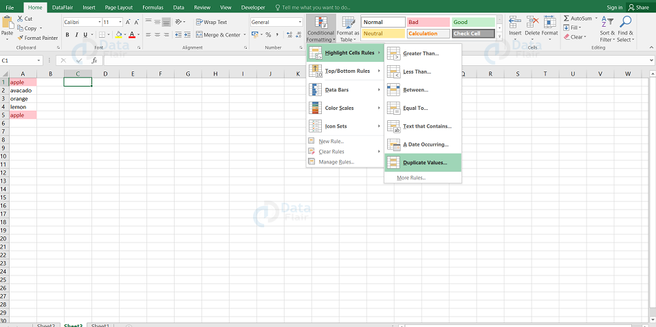
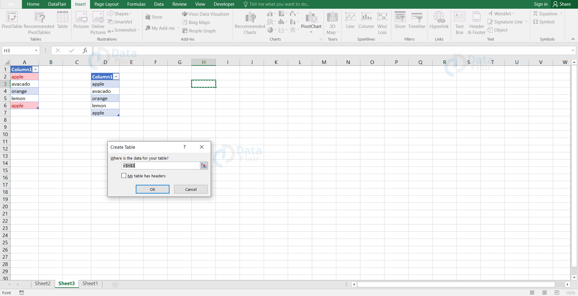
13. What are the possible ways to find the duplicate values in a column?

There are two ways to fetch the duplicate values in a column and they are conditional formatting or by making use of the countif function.

1. Conditional Formatting:
To make use of the conditional formatting, click on the home tab and choose “Highlight cell rules”. Then, finally click on the “Duplicate values” option.

2. Countif():
The user can make use of the countif function to check whether the values in a particular column are repeated.

14. You need to create a single variable in a code and store multiple names in it. Is that possible to do?

Yes, we can do it by creating an array. The following code is a sample of it.

Private Sub Student_names()
   Dim arrNames(0 to 3) as String  
     arrNames(0) = "Vihaan" 
     arrNames(1) = "Arjun" 
     arrNames(2) = "Arya"
      arrNames(3) = "Shrishta"
 
 End Sub

15. What is the role of nested if condition and write its syntax?

Nested IF:
The nested if condition is a function which contains a lot of IF statements inside an IF function and it is used to evaluate in excel when there are more than one condition to be looked after in a dataset. It can also be said that it is a function which starts with an IF function and the other IF functions are added inside the original IF function.
Nested IF Syntax:

=IF(logical_test,[value_if_true],[value_if_false],IF(logical_test,[value_if_true],[value_if_false], ...))

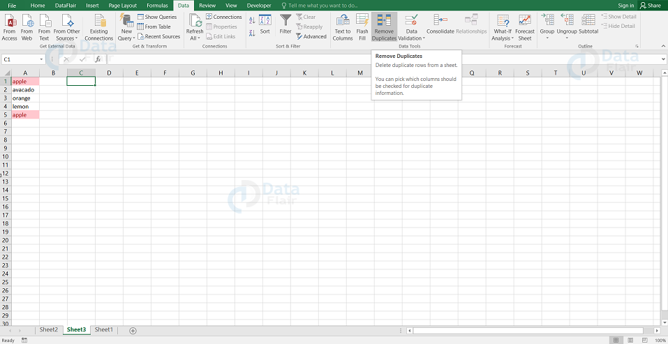
16. How can a user remove duplicate values in a range of cells?

To delete duplicate values in a column, choose the highlighted cells from conditional formatting and press the delete button from the keyboard. After deleting the values, go to the ‘Conditional Formatting’ option under the Home tab. Select ‘Clear Rules’ to remove the rules from the excel sheet.

The user can also delete duplicate values by choosing the “Remove Duplicates” option under the Data tab.

17. What is the formula you can use to fetch data from the dataset?

In order to fetch the data from a dataset, we can use the vlookup function. For example, if we are fetching a particular mark in a student mark list then we have to mention the student’s name, table range, the column number, match type “=VLOOKUP(Akkshaya, A2:D25, 3, 0)” . Here 0 represents the exact match.

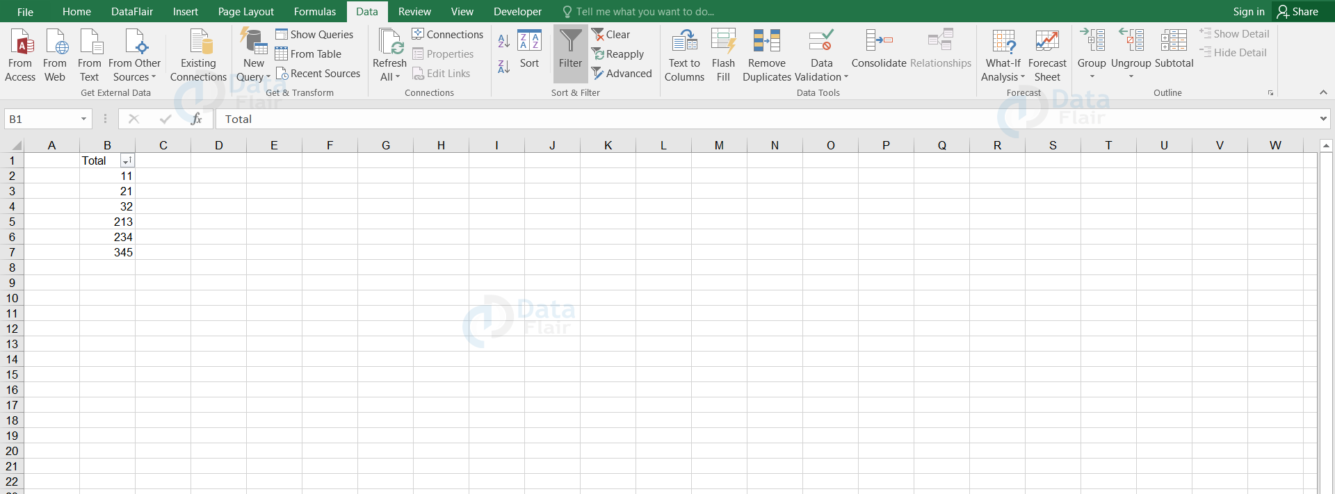
18. Can we filter or sort the data from smallest to largest?

Yes, we can filter the data as per the requirement. To sort the data from smallest to largest, click on the filter options under the data tab. Then, select the smallest to highest option from the drop down list beside the header cell.

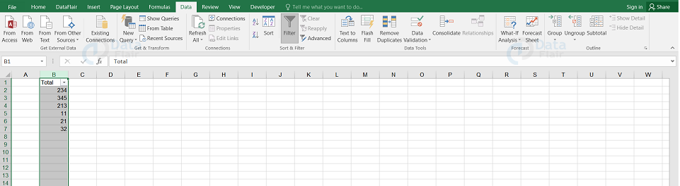
After choosing the option, the following result appears

19. How to create a “not equal to” operation case in VBA?

Sub Notequal_Click()
    Dim a As Integer, b As Integer
    num1 = 100
    num2 = 100
    If a <> b Then
            MsgBox ("True")
        Else
            MsgBox ("False")    
    End If
End Sub

20. Can we use a logical operator in VBA code and if so, give me a sample?

Private Sub log_operator()
Dim num1 As Integer, num2 As Integer, output As String

num1 = 100
num2 = 200

If num1 >= 100 Or num2 > 200 Then
    output = "The output cleared the logical function"
Else
    output = "It did not pass the condition"
End If

Range("C1").Value = result

End Sub

Advanced Interview Questions on MS Excel

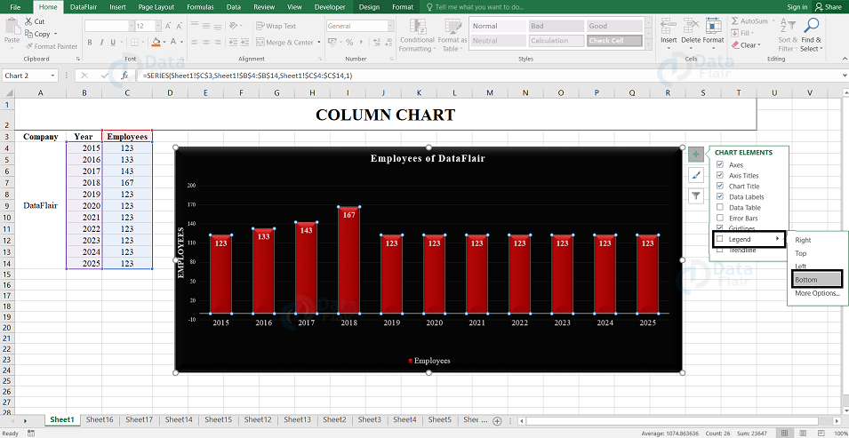
21. What are the steps to change the legend position in the chart?

The legend position can be changed as per the user’s convenience through below steps:

1- To change the legend position, click on the chart and then select the “+” symbol from the right side of the chart.

2- From there, go to legend and click on the arrow beside it.

3- Finally, choose on which side it has to appear. The changes will be reflected on the chart.

22. When we could use variables for each element, why do we go for a VBA array?

We choose the VBA array because it helps in grouping logically related data. For example, if we wanted to save employee records then we can use an array variable with separate location for each category. It is easy to maintain the codes as we use only one variable instead of many variables. Retrieving, sorting and modifying the data in an array is faster and this also means it has a better performance.

23. How do reports and dashboard vary in Excel?

Reports: We use the historical data to form reports and reports include visuals such as tables, graphs,charts and texts etc. The reports that are made are not live.

Dashboards: The dashboards we create in excel are dynamic and live. When we change or update the data in dashboards, the visuals will also be altered and we can see the changes. Dashboard also contains visual displays such as tables, charts and values etc.

24. Write the code to create a textbox in VBA?

Private Sub TextBox_Mdo()
TextBox.Text = "We have created a textbox via code!"
End Sub

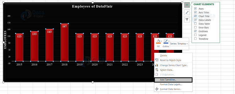
25. What are the steps to add a trendline in the chart?

The steps to follow to add a trendline are:

1: Click on the chart, then at the right side of the chart click +.

2: Click on the arrow present next to the trendline and choose more options.

3: The format trendline pane will now be visible. Then choose an option from the trendline pane.

4: Select linear trendline options, then to include in the forward forecast specify the number of periods.

5: Finally check mark on display equation on chart and display R-squared value on chart option.

26. Is there any smart way to return to a particular area of a worksheet?

We can return to a specific area of a worksheet by referencing the specific area by name box. When we type the range name on the cell address, it takes us to the specific area of a worksheet.

27. Can we debug a macro code?

Yes, we can debug a macro code and this situation comes when there are chances of users to commit mistakes in the code and that leads to error. So to overcome the error in the code, we can debug the code just as we do to any other coding language. We can also know about the errors and eventually we can correct them.

To debug a macro code, click on the macros option under the developer tab and select the “step into” option from the box. Once you select it, the code automatically opens up in Microsoft Visual Basics for Applications.

28. Can we provide Dynamic Range in ‘Data Source’ of Pivot Tables?

Yes, we can provide the data source in dynamic range for the pivot tables. When we provide it dynamically, the table automatically adds the new records in the summary and we can see the changes once the table is refreshed. To provide the range, select the table under the insert tab and give a name to the table if you want.

29. Write a code using a function to calculate the quadrant of a number in VBA

Function quadrant (ByVal my_num As Integer) As Integer
 my_num =  my_num *  my_num
quadrant =  my_num
msgbox(“The quadrant value of a number is:” quadrant)
End Function

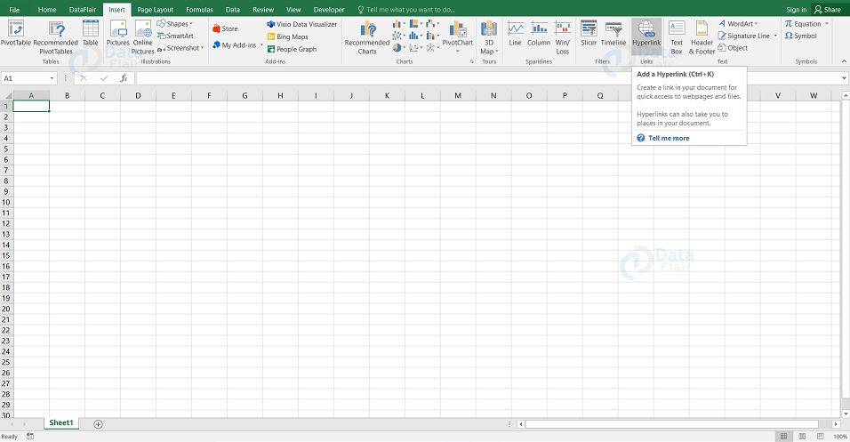
30.Can we create hyperlinks in Excel? What is the procedure to insert it?

Yes, we can create hyperlinks in excel. Hyperlink is a function which helps the user to open the document stored in that particular link and we can also use hyperlinks to navigate in and between the sheet also.

In order to insert a hyperlink in excel, go to the hyperlink option under the insert tab. When you click on it, the list of files and documents appear, we can either choose from it or we can just browse for the required information.

Summary:

This article would help the candidate to clear the doubts about Microsoft Excel interview questions and will also be very helpful to crack the interviews.