Grouping in Excel | Filters in Excel
Placement-ready Courses: Enroll Now, Thank us Later!
In this tutorial, let’s have a brief idea about what is filters and grouping in Excel.
Grouping in Excel
Groupings in Excel helps to hide the rows and columns of the data records and it also helps in summarizing the grouped data records.
Grouping in MS-excel is one of the tactics each and every excel expert and financial analyst should know. Financial analysts should know about this to make their financial sheet much clearer and understandable.
To access grouping in MS-Excel, follow the steps:
1: Click on the data tab.
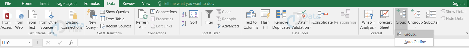
2: Choose the cells.
3: Choose groups from the menu.
4: A box appears with the option of rows and columns.
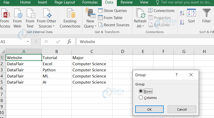
5: Choose the ones you wanted to group either rows or columns.
6: Click ok.
Note: When we click on rows, then it hides the whole row and we will also get 2 states for each group on the side of the spreadsheet.
Have a look at the sample to understand it more clearly.
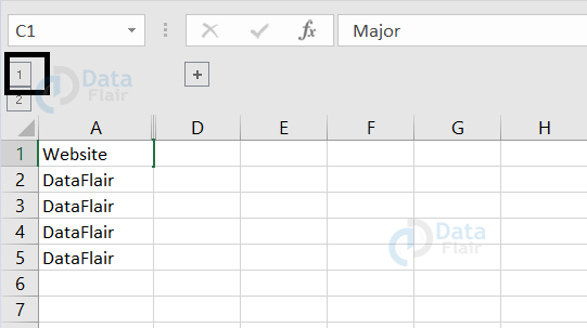
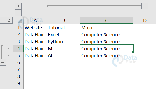
We have chosen the cell A4, A5 for grouping row-wise.
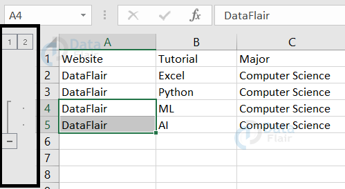
The 1 and 2 numbers apart from the serial number are the state numbers. Each state number performs different actions.
If you click on 1, it hides the grouped data.
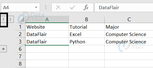
Hope you noticed the serial number after 3 is 6.
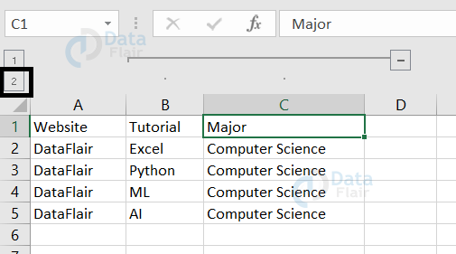
If you click on 2, it unhides the grouped data.
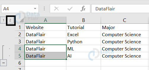
Hope you saw the dots near the serial number 4 and 5. These dots indicate that they are grouped together and once when we click 2, the data is unhidden.
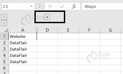
When you click on the ‘-’ symbol it hides the data and changes the symbol to +. It indicates that we can unhide the data by clicking on the + symbol.
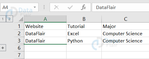
Here also, we can see that row 4 and row 5 are not visible as hiding takes part.
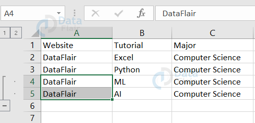
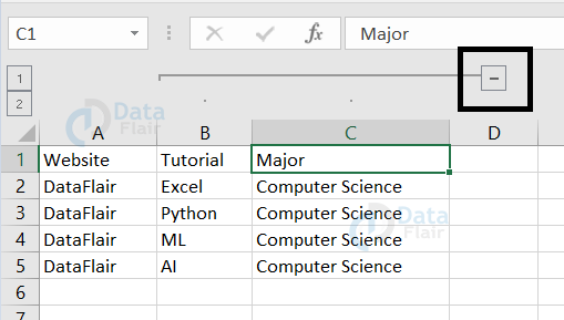
By clicking on the + symbol, the data is unhidden.
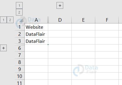
Now, let’s have a look at how the group works if we choose the column option in the box.
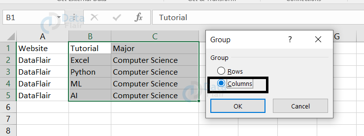
It hides the whole column if we choose the ‘columns’ group, the dots are now seen above the columns.
Observe that state number 1, 2 are now visible above the columns. Once we press the state number 1, the D column follows the A column hiding the B and C columns.
Once we press state number 2, the grouped columns will appear back in the spreadsheet.
Look at the – and + symbols. It also works as such in the rows grouping but this time it hides the columns. Let’s look at the sample:
When we press on the – symbol, the symbol changes back to the + symbol. It indicates that the columns are hidden are ready to revert back anytime.
Now, when we press on the + symbol, the B and C columns are visible.
Another interesting fact is that we can also group inside a group. Let’s have a look at the sample to form a group inside a group.
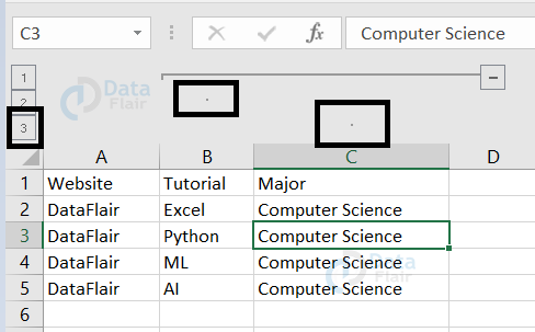
The ‘.’ symbol in column c is corresponding to state 3 which means it is being grouped inside a group.
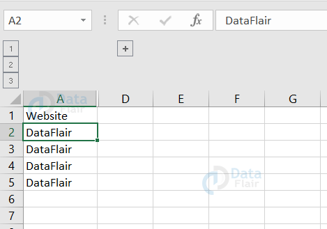
Now, let’s have a look at how it works. When we press the state 1, the column B and C are temporarily hidden.
When we press state 2, the c column is alone hidden.
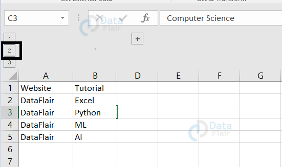
Observe that the D column follows column B hiding column C.
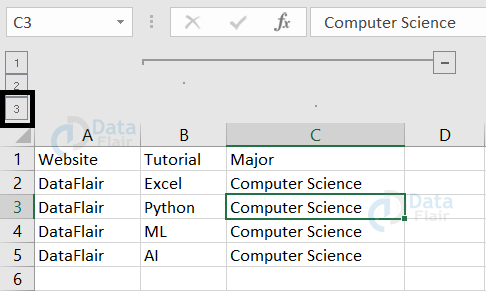
When we press state 3, the c column is again visible.
This is how grouping inside a group works. Now, let’s have a look at the grouping of rows and columns together.
In this case, when we press the – symbol on both sides, the rows, as well as the columns, will be hidden.
Observe that the – symbol is being changed to +.
After the number 3, the number 6 has come, depicting that rows 4 and 5 are hidden. Also, after the A column, the D column is being followed depicting the temporary hiding of B and C columns.
Ungrouping in Excel
Ungroup is a feature that helps in ungrouping the cells which were once grouped.
To apply ungroup, follow the steps:
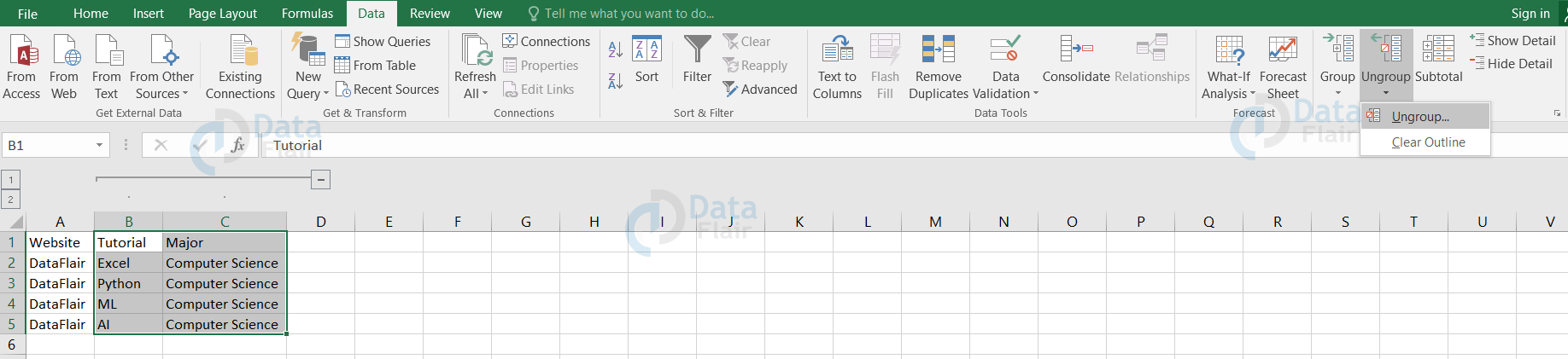
1: Click on the DATA tab menu.
2: Choose the ungroup option from the ribbon.
3: Choose either its row or column.
4: Click on it.
Let’s understand looking at a sample:
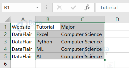
Hope, you noticed that the state numbers and the dot above the B and C columns are being removed. This means that the grouped cells are ungrouped using the ungroup option.
Subtotal in Excel
Subtotal is a feature that helps in deriving the subtotal for your data values in the spreadsheet. To apply subtotal to your dataset, follow the steps:
1: Click on the cells in the spreadsheet.
2: Click on the data tab menu.
3: Choose subtotal from the ribbon.
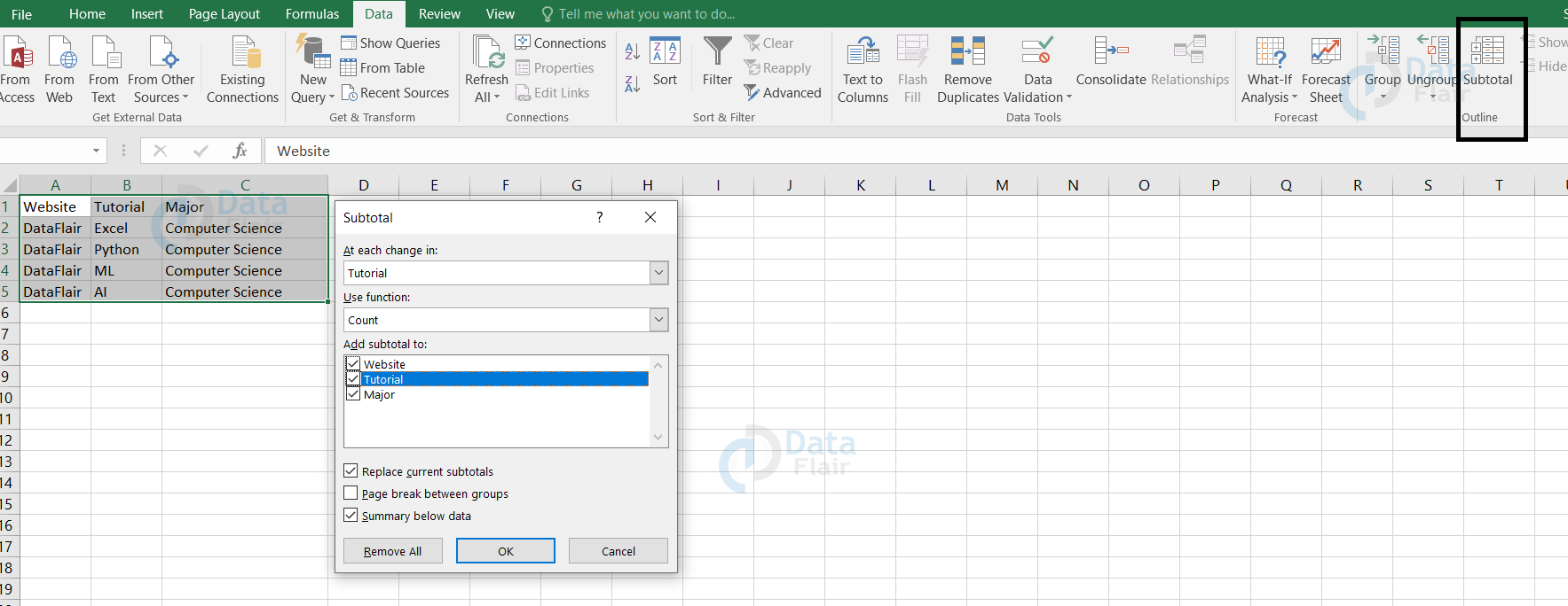
A box appears asking for- at each change in, use function, add subtotal to.
- At each change in – This function brings a subtotal after each change in that particular attribute.
- Use function – It asks for which type of function to apply on those cells.
- Add subtotal to – This option is being displayed with a box along with the headers in the dataset. You can choose which all header, the subtotal should appear.
There are another 3 checkboxes. Check the boxes once you feel like it’s necessary and those options are- replace current subtotals, page break between groups, and summary below data.
Replace current subtotals: It keeps replacing the subtotals.
Page break between groups: This provides a page break between groups and is viewed in PDF only.
Summary below data: This provides you the summary below the groups.
Let’s understand this feature with a sample:
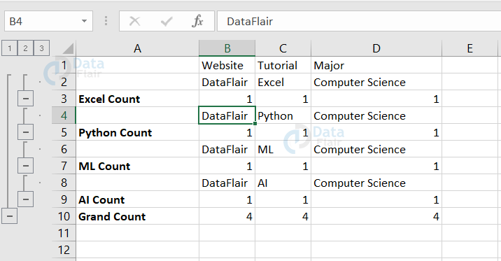
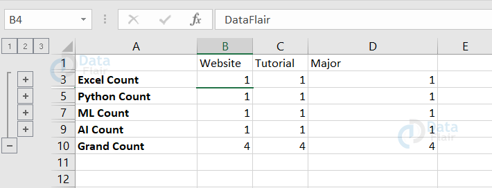
From the sample, we can understand that for each change in the tutorial, the function is being applied.
The ‘-’ symbol helps in hiding the details of the dataset. It provides only the subtotals of that particular group and once the ‘-’ symbol is being clicked, it’s converted to ‘+’.
Let’s see a sample:
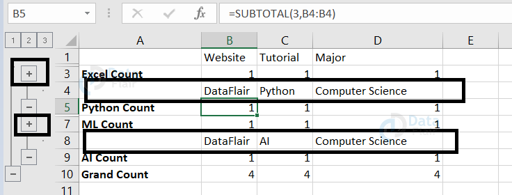
Once we click on the ‘-’ symbol beside row numbers 3 and 7, it’s converted to ‘+’ and only the subtotals are visible in the spreadsheet. The datasets for those particular groups are not visible in the spreadsheet since they are being hidden.
The rows corresponding to the ‘-’ symbol contain the details of the particular group and also the subtotals.
The state numbers are 3 in this case.
If we press 1, only the grand total appears.
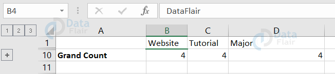
When we press 2, the subtotals alone appear.
If we press 3, the dataset appears along with the subtotal.
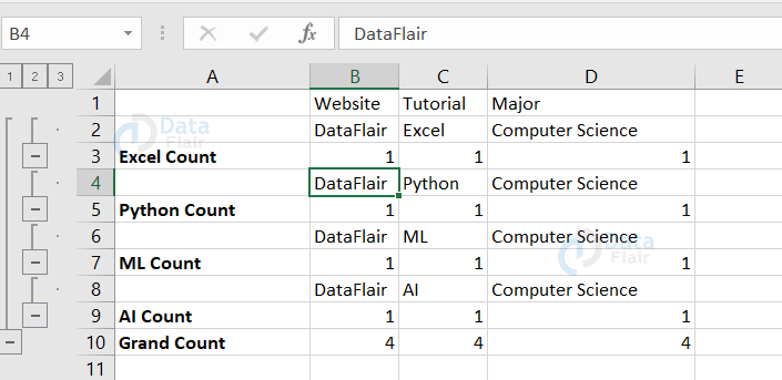
This is how subtotal works on the spreadsheet.
Now, let’s get into the features of filters in MS-Excel.
Filters in Excel
Filtering in Excel helps to hide the data records temporarily. It also helps in focusing on certain records which meet the condition criteria by hiding the other data in the spreadsheet.
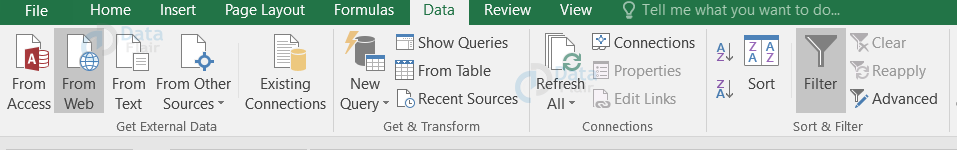
To apply filters on the dataset, follow the steps:
1: Place the cursor on a cell.
2: Go to the DATA tab.
3: Apply filter from the menu.
Once you click the filter, the header in the dataset appears with a dropdown menu.
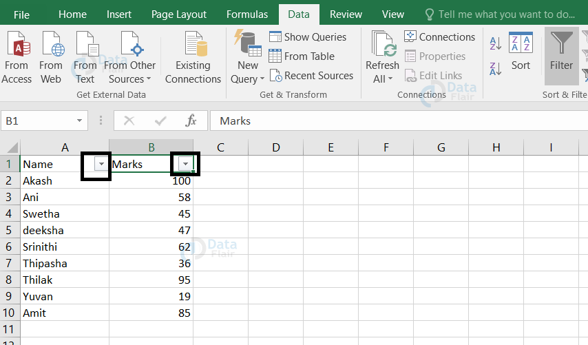
Once you click on the dropdown, it shows a box with different functions.
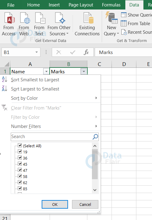
The main functions that are performed by filters are sorting and number filters.
The values below search are the data values provided in the spreadsheet. We can also make use of the search tab to search for particular data.
If you wanted to view some of the data, then uncheck the box beside ‘select all’ and choose whichever data you wanted to view.
Let’s now, look at how the sorting works.
Sort Smallest to Largest in Excel
When you click on it, the data appears from the smallest value to the largest value.
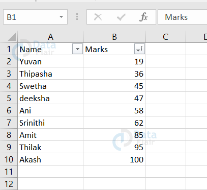
From the above sample, we can see that the marks are being arranged in ascending order and the names are also shifted according to the replacement of the marks.
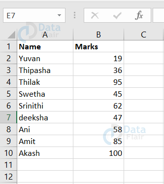
Sort Largest to Smallest in Excel
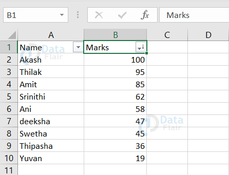
From the above sample, we can see that the marks are being arranged in descending order and the names are also shifted according to the replacement of the marks.
Types of Data Filters in Excel
Data filters can be applied on different data types such as:
- Text values
- Numeric values
- Date values
Let’s look at a sample:
1. Text Values in Excel
Filters can perform their task even on the text data types.
In the above sample, we are going to sort the names from A to Z. Let’s now apply a filter and try it out.
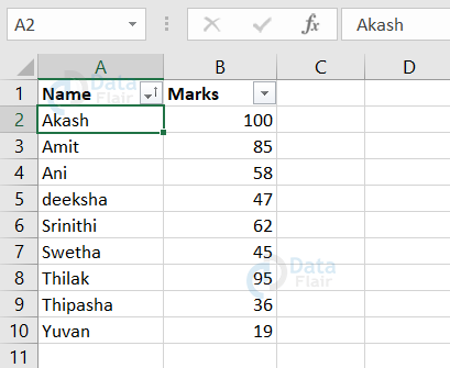
Hope, you all noticed that the names are being arranged from A to Z using filters.
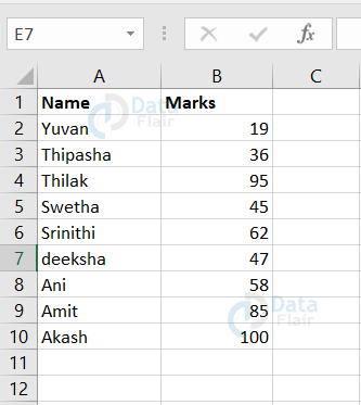
2. Numeric values in Excel
Filters perform their task even on the numeric data types.
In this sample, we are going to arrange the marks in ascending order using filters.
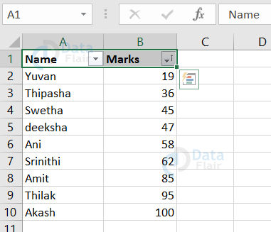
Hope, you observed that the marks column is being arranged in ascending order using the filter options.
3. Date Values in Excel
The filters perform the task on the date column also. Let’s look at a sample to understand it more clearly.
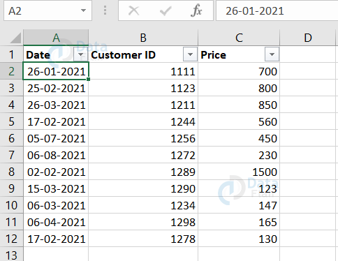
In this sample, we are going to arrange it from the oldest to newest in the date column.
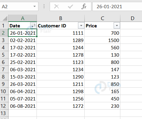
From the above sample, we can see that the dates are arranged from the oldest to the newest using filters.
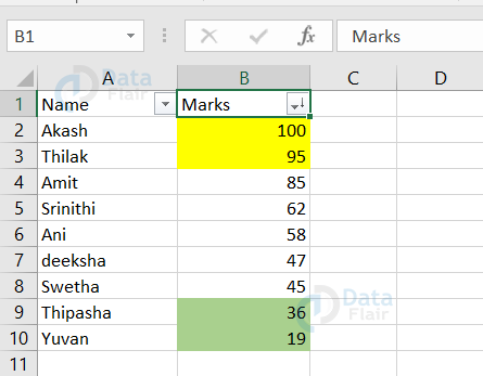
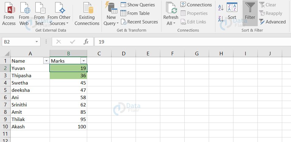
Filter by Colors in Excel
The values which are being colored will appear when we filter by the color differentiation.
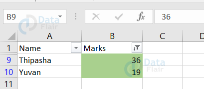
In the sample, the students whose marks are very low are being colored green and using filters by colors, the excel provides that particular data alone.
Notice that the other cells are temporarily hidden. After row number 1, it is being followed by row number 9 and 10.
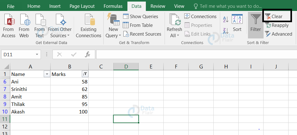
Clear filter in Excel
If you have applied a filter to the header, then the clear filter activates. This means that if you wanted to remove the filter from the header, then you can just click on it. Once you click, the filter will be removed by which all the unhidden data records will be visible back again.
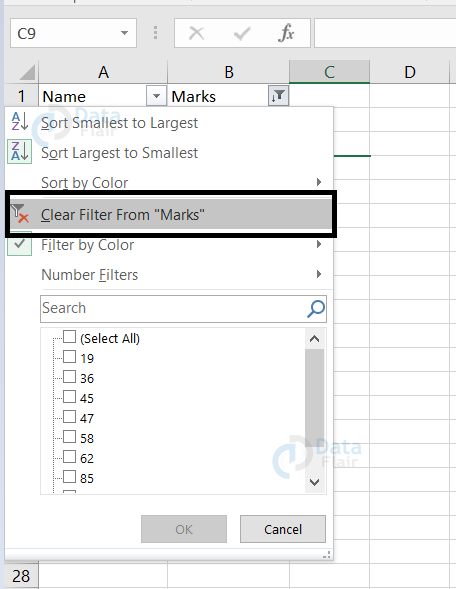
Hope, you can notice that the clear filter from marks is being activated, once you click on it.
The whole data records in the spreadsheet are now visible back again.
Now, let’s have a look at the Number Filters and the options available in it.
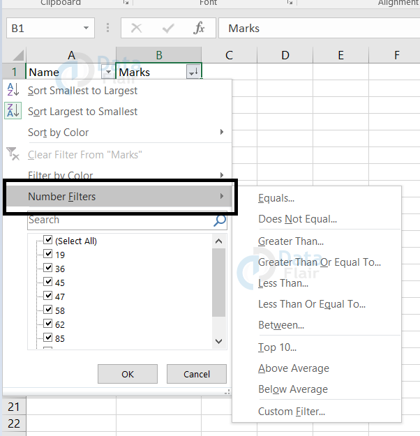
The number filters contain options like the comparison operators.
Let’s look at the table below to know how each option performs:
| Option | Function |
| Equals | It displays the data records equal to the value provided in the box and hides the remaining records. |
| Does Not Equal | It displays the data records that are not equal to the value provided in the box and hides the remaining records. |
| Greater than | Displays the records which are greater than the value specified in the box. |
| Greater than or Equal to | Displays the records which are greater than or equal to the value specified in the box. |
| Less Than | Displays the records which are lesser than the value specified in the box. |
| Less than or equal to | Displays the records which are lesser than or equal to the value specified in the box. |
| Between | Displays the records which are in between the maximum and minimum value specified in the box. |
| Top 10 | Displays the top 10 records of the spreadsheet. We can also view more or less than 10 numbers of records. Here the n can be of any value like n=1, 3, 25. |
| Above Average | Displays the records which are above the average. |
| Below Average | Displays the records which are below the average. |
| Custom Filter | Displays the records as per the user convenient as the user will be providing the constraint. |
How to copy paste a filtered data in Excel
Now, let’s look at how to copy paste the filtered data.
1: Place the cursor on the cell.
2: After applying the required filter, click Ctrl+A
Note: Ctrl + A selects all the data records.
3: Click Ctrl+C to copy the data.
4: Go to the sheet where you want to paste, then click Ctrl+V.
Now, you can see your filtered data in the desired sheet. Let’s look at an example below:
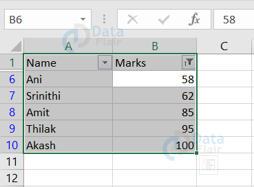
In this sample, the filter fetches the data records of the students with marks above 50.
Click on ctrl+a to choose all the filtered cells and then click on ctrl+c for copying the records.
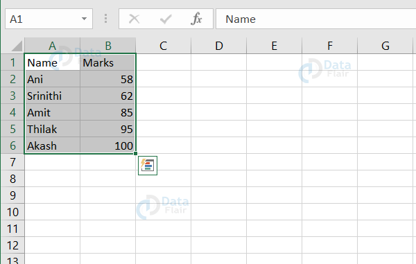
Then, go to the required sheet and press ctrl+v to paste the data.
Let’s look at the menu filter options. There are clear, reapply and advanced filter options.
After applying the filter, the clear and re-apply menu will be clickable. When you click on clear, then the removal of the filter takes place.
From the sample, we can see that the filter is removed and the clear filter is not available now.
Reapply in Excel
The reapply helps in reapplying the sort or filter of the records and this can be done whenever you open the spreadsheet.
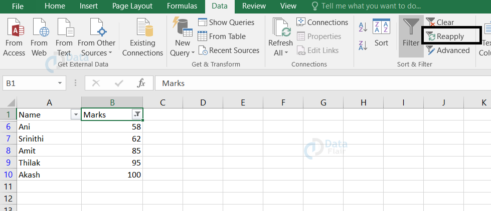
Once you click on the reapply option, then the sort or filter criteria will be reapplied to the data records.
Advanced Filters in Excel
In advanced filters, the data records apply filters in another location also. It can be either in the same worksheet or in the new worksheet. In basic filtering, we cannot filter the data records anywhere else other than the source data.
To do advanced filtering, follow the steps:
1: Click on the DATA tab.
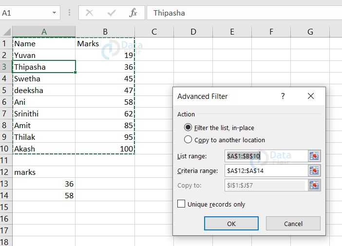
2: Click on the advanced filtering option. A box appears.
3: Press OK after filling the box.
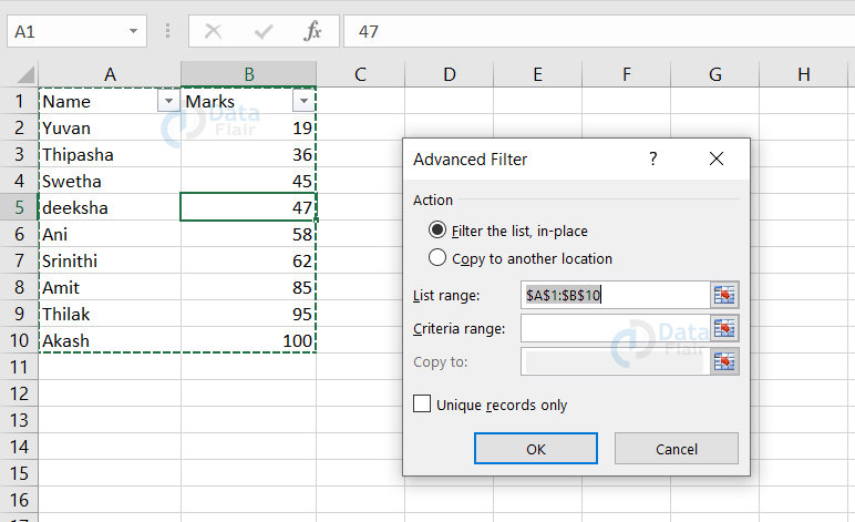
List range in Excel
Once we click on the advanced filter, the list range is automatically filled.
The data records that are being considered in the list range are shown in the dash lined box.
Criteria range in Excel
After making sure the list range, click on the criteria range and choose the range which should be filtered from the total data records.
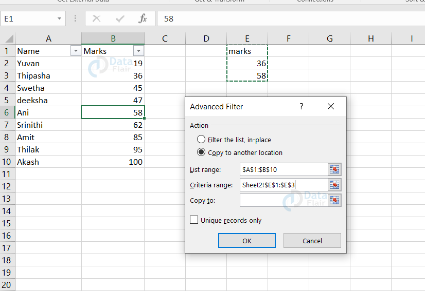
In this sample, we are going to filter the students with the marks 36 and 58.
Copy to in Excel
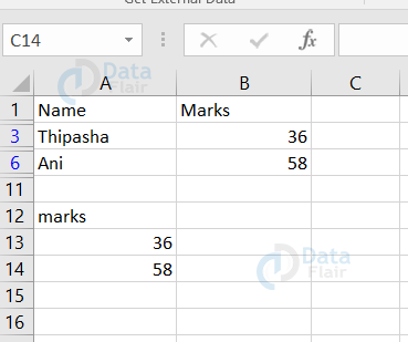
The copy to function activates only after the user chooses the ‘copy to another location’ radio box. Once done, then select the range of cells where the filtered data should appear.
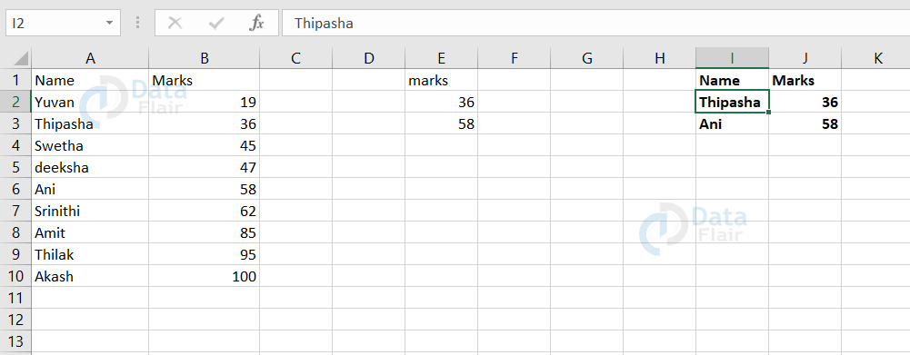
From the above sample, we can observe that the filtered data records are visible in the destination provided.
Or else, if we have chosen ‘filter the list, in-place’ radio box option, then the data will be filtered in the source data place itself.
In this sample, the filter applies in the list range itself.
Hope, you have observed that the data are filtered in the source data place itself.
Summary
The filters help in focusing a particular set of data records by hiding the other data records in the spreadsheet. Groups in MS-Excel help the user to group and hide the required rows and columns in a spreadsheet.
You give me 15 seconds I promise you best tutorials
Please share your happy experience on Google


Hammad