Greedy Algorithm of Data Structures
Learn DSA & Get Ready for MAANG Companies Start Now!!
Ever wondered how an ATM works? After swiping your card and entering your pin, it asks you to enter the amount you need to withdraw. Now, ATMs have a greedy algorithm that forces these machines to choose the largest denomination possible.
Suppose there are denominations of ₹100, ₹200, ₹500, and ₹2000 in a machine and you want to withdraw ₹7300. Then the greedy approach opted by ATM will be:
- Select three ₹2000 denomination notes. Remaining amount ₹1300
- Select two ₹500 denomination notes. Remaining amount ₹300
- Select one ₹200 denomination note. Remaining amount ₹100
- Finally, select ₹100 denomination note and this solves the problem.
In this article, we will learn about the greedy algorithms, their properties, and the steps to achieve a greedy algorithm design. We will also see some real-life examples of greedy algorithms.
Greedy Algorithm
Greedy algorithms find out many possible solutions and choose the best solution for the problem. In this algorithm, we focus on the individual sub-models of a bigger problem and we try to solve them independently.
- Each step-by-step solution must approach the problem towards its best solution possible.
- It may not give an optimal solution.
- The problem where there is no optimal solution possible, the greedy algorithm provides us with a solution that is close to optimal.
History of Greedy Algorithm
- Edsger Dijkstra proposed the concept of greedy algorithms to generate minimum spanning trees. He wanted to short the routes in Amsterdam.
- Greedy algorithms were used for multiple walk graph problems in the 1950s.
- American researchers, Cormen, Rivest, and Stein in 1970 put forward a proposal for recursive substructuring of greedy solutions in their book “ Introduction to algorithms”.
- Many networking protocols like open-shortest-path-first (OSPF) use a greedy approach to minimize time spent on the network.
Properties required for the Greedy Algorithm
A greedy algorithm works if the problem is having the following two properties :
- Greedy choice property: We can reach a globally optimized solution by creating a locally optimized solution for each sub-module of the problem.
- Optimal substructure: Solutions to subproblems of optimal solutions are also optimal.
Characteristic of a Greedy Approach
- The resources available have costs attached to them. These are the constraints.
- The greedy approach uses maximum resources in time a constraint applies.
Steps to achieve Greedy Algorithm
- Feasible: The algorithm should follow all constraints to return at least one solution to the problem.
- Local optimal choice: Make optimum choices from currently available options.
- Unalterable: We cannot change a decision at any subsequent point while execution.
Advantages of Greedy Algorithm
- Very few trade-offs compared to other algorithms, make it highly optimized.
- The best solution is reachable immediately since multiple activities can execute in a given time frame.
- No need to combine the solutions of subproblems.
- This algorithm is very easy to describe.
Failed Greedy Algorithm
Let us change the above example by a bit. Let us assume that we now have only denominations of ₹100, ₹700, and ₹1000. Now if we use the greedy algorithm, to withdraw ₹1500, we will get one ₹1000 denomination note and five ₹100 denomination notes. Total 6 notes.
But this is not an optimal solution. If we get two ₹700 denominations and one ₹100 denomination, we can achieve the task in just 3 notes. This proves that a greedy algorithm does not always provide us with an optimal solution.
Therefore in such cases, the Greedy method can be wrong and sometimes in the worst case even results in a non-optimal solution.
Applications of Greedy Algorithm
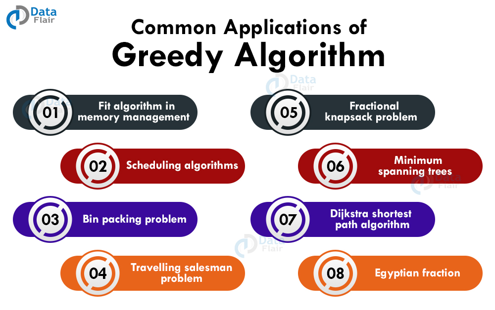
1. Fit algorithm in memory management
Fit memory management algorithms are techniques for allocating the memory blocks to the processes in an operating system.
Here, a pointer keeps track of all the memory blocks and accepts or rejects the request of allocating a memory block to an incoming process. There are three types of fit memory management algorithms:
- First fit algorithm: First sufficient memory block from the top of the main memory is allocated to the process.
- Best fit algorithm: Minimum sufficient memory block available in the memory is allocated to the process.
- Worst fit algorithm: Largest sufficient memory block available in the memory is allocated to the process.
2. Scheduling algorithms
A typical process in a computer has input time, output time, and CPU time. In multiprogramming systems, while one process is waiting for its input/output the other processes can use the CPU.
Process scheduling algorithms perform these tasks. These algorithms determine which process will use the CPU for execution and which processes will be on hold. These algorithms make sure that the CPU utilization is for maximum time and process execution takes place in minimum time.
Six types of scheduling algorithms are:
a. First come first serve: In this non-preemptive scheduling algorithm, the processes are executed on a first come first serve basis.
b. Shortest job first: In this non-preemptive scheduling algorithm, the approach is to minimize the waiting time for the process.
c. Priority scheduling: This non-preemptive algorithm assigns each process a priority, and the process with the highest priority is executed first.
d. Shortest remaining time: In this preemptive scheduling algorithm, the process which has the least time remaining for its completion is executed first.
e. Round robin scheduling: In this preemptive process scheduling algorithm, each process is provided a fixed time to get executed. If the process is not completely executed, it will be assigned the same time for execution in the next round.
f. Multiple level queue schedule: These are not independent scheduling algorithms. Programmers make many queues for processes with common characteristics and every queue can have its own scheduling algorithm.
3. Bin packing problem
We need to pack items of different volumes into a finite number of bins of fixed volume each in such a way that we use the minimum number of bins. Placing data on multiple disks and loading containers like trucks are some real-life examples of this algorithm.
4. Travelling salesman problem
Given a set of cities and distance between every pair of the city, the objective is to find the shortest possible path to visit each city exactly once and return to the starting point.
5. Fractional knapsack problem
Imagine you have different items with their weights and their values. Our objective is to determine the subset of items that we should include in a collection so that their total weight is less than or equal to a given limit and their value is maximum. The fractional knapsack problem is an optimization problem.
6. Minimum spanning trees
Minimum spanning tree is a subset of the edges from starting to end in a weighted and undirected graph. MST connects all vertices without any cycle and the total weight of all the edges included is minimum..
7. Dijkstra shortest path algorithm
Finding the shortest path between two vertices in a graph such that the sum of weights between the edges is minimum.
8. Egyptian fraction
We can represent every positive fraction as a sum of unique unit fractions. For example, the Egyptian fraction representation of 47/154 is 1/7 + 1/11 + 1/14.
Problems solved by the Greedy Approach
1. Activity search problem
The activity search problem is a mathematical search optimization problem. This is used in scheduling a single resource among several ongoing and incoming processes. A greedy algorithm provides the best solution for selecting the maximum size set of compatible activities.
Let S = {1,2,3,…n) be a set of n proposed processes. Resources can be used by only one process at a time. Start time of activities = {s1,s2,s3,….sn} and finish time = {f1,f2,f3,…fn}. Start time is always less than finish time.
If activity “i” starts meanwhile the half-open time interval [si, fi), then, activities i and j are said to be compatible if the intervals (si, fi) and [si, fi) do not overlap.
Algorithm:
activity_selector (s, f)
Step 1: n ← len[s]
Step 2: A ← {1}
Step 3: j ← 1.
Step 4: for i ← 2 to n
Step 5: do if si ≥ fi
Step 6: then A ← A U {i}
Step 7: j ← i
Step 8: return A
Example :
S={A1,A2,A3,A4,A5}
si={1,1,2,3,4}
fi={4,2,4,7,6}
Step 1. Arrange in increasing order of finish time.
| Activity | A2 | A3 | A1 | A5 | A4 |
| si | 1 | 2 | 1 | 4 | 3 |
| fi | 2 | 4 | 4 | 6 | 7 |
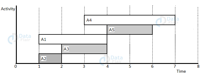
Step 2: Schedule A2
Step 3: Schedule A3 (A2, A3 not interfering)
Step 4: Skip A1 (Interfering)
Step 5: Schedule A5 (A2, A3, A5 not interfering)
Step 6: Skip A4 (Interfering)
Step 7:Final Activity schedule is A2, A3, A5.
2. Fractional Knapsack Problem
Optimization problem where it is possible to select fractional items rather than binary choices of 0 and 1. The binary problem cannot be solved by a greedy approach.
Step 1: Calculate the value per pound.
Step 2: Take the maximum possible amount of substance with the maximum value per pound.
Step 3: If that amount is exhausted, and we have space, take the maximum possible amount of substance with the next maximum value per pound.
Step 4: Sort the item values per pound, greedy algorithm has a time complexity of O(n log n ).
Algorithm:
fractional knapsack (Array w, Array v, int C)
1. for i= 1 to size (v)
2. do vpp [i] = v [i] / w [i]
3. Sort-Descending (vpp)
4. i ← 1
5. while (C>0)
6. do amt = min (C, w [i])
7. sol [i] = amt
8. C= C-amt
9. i ← i+1
10. return sol
Example:
I = { I1,I2,I3,I4}
w={ 20,30,40,50}
v={40,20,70,60}
Capacity, C = 75
Step 1: vpp = { 2,0.66,1.75,1.2}
Step 2: Choose I1. Total weight 20. Left Capacity = 40
Step 3: Choose I3, Total weight 40. Left capacity = 15
Step 4: Choose I4 fractional. Total weight 15. Left capacity = 0
Step 5: value = 40+70+1.2*15 = 128
3. Huffman Coding
Huffman coding is used for efficient data encoding for data compression problems.
For example, there are 106 characters in a file but only a few characters appear repeatedly :
| Character | a | e | i | o | u |
| frequency | 45 | 13 | 12 | 14 | 16 |
Expressing the file in a compact way:
- Fixed length Code: each character is represented by 3 bits per character. For the whole file, we will need 3 x 106 bits.
- A variable-length code: it assigns long bits for infrequent characters to generate and short bits for frequent characters.
| Character | code |
| a | 0 |
| e | 101 |
| i | 110 |
| o | 100 |
| u | 111 |
Total bits required: ( 45*1+13*4+12*4+14*3+16*3 )*1000 = 210,000 bits.
Prefix codes
Prefixes of one encoded character cannot be complete coding to any other character. For example, 100 and 1001 are not valid codes because 100 is a prefix to a code. Prefix codes make encoding and decoding very comfortable.
Algorithm :
huffman (C)
1. n=|C|
2. Q ← C
3. for i=1 to n-1
4. do
5. z= allocate-Node ()
6. x= left[z]=Extract-Min(Q)
7. y= right[z] =Extract-Min(Q)
8. arr [z]=arr[x]+arr[y]
9. Insert (Q, z)
10. return Extract-Min (Q)
4. Travelling Salesman Problem
Given a set of cities and distance between every pair of the city, the objective is to find the shortest possible path to visit each city exactly once and return to the starting point.
Let there be n cities named, x1,x2,x3,…..xn. Cij is the cost of traveling from xi to xj. Find the route starting and ending at x1, going through all cities for minimum cost.
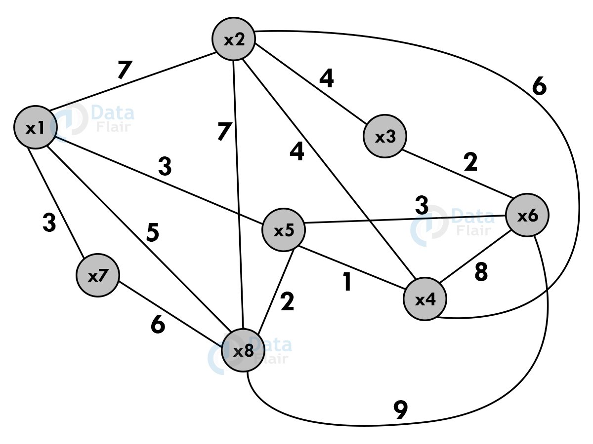
Cost adjacency matrix:
| x1 | x2 | x3 | x4 | x5 | x6 | x7 | x8 | |
| x1 | 0 | 7 | 0 | 0 | 3 | 0 | 3 | 5 |
| x2 | 7 | 0 | 4 | 6 | 0 | 0 | 0 | 7 |
| x3 | 0 | 4 | 0 | 0 | 0 | 6 | 0 | 0 |
| x4 | 0 | 6 | 0 | 0 | 1 | 8 | 0 | 0 |
| x5 | 3 | 0 | 0 | 1 | 0 | 3 | 0 | 2 |
| x6 | 0 | 0 | 6 | 8 | 3 | 0 | 0 | 9 |
| x7 | 3 | 0 | 0 | 0 | 0 | 0 | 0 | 6 |
| x8 | 5 | 7 | 0 | 0 | 2 | 9 | 6 | 0 |
Shortest path : x1 -> x5 -> x4 -> x2 -> x3 ->x6 -> x8 ->x7 -> x1
Cost : 3 + 1 + 6 + 4 + 6 + 9 + 6 + 3 = 38
5. Kruskal algorithm
A minimum spanning tree algorithm finds the subset of graphs which:
- Forms a tree including every vertex.
- Has minimum sum of weights among all trees that are possible in a graph
- Kruskal’s algorithm checks if adding an edge creates a loop or not.
Algorithm:
- Sort all edges in ascending order of their weights.
- Add the edge with the lowest weight to the spanning-tree
- Keep on adding edges until all the vertices are included.
For example:
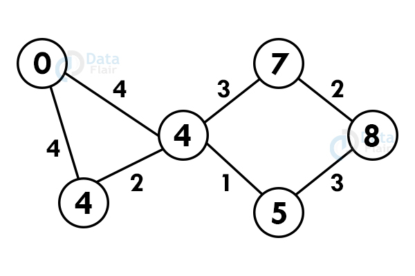
Using Kruskal’s algorithm, create a minimum spanning tree of the following graph:
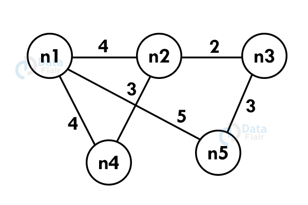
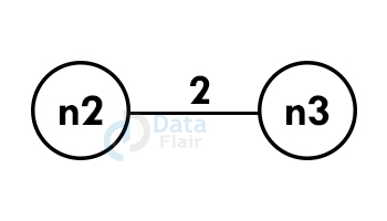
Step 1: Select an edge with the minimum. If the graph is having multiple minimum weighted edges, you can select any of them.
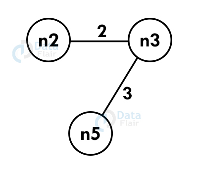
Step 2: Select the next shortest edge and add it to the tree.
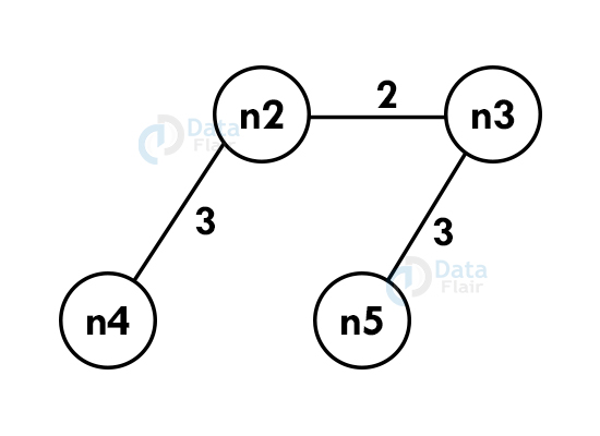
Step 3: Select the next shortest edge and add it. The edge should not create a cycle.
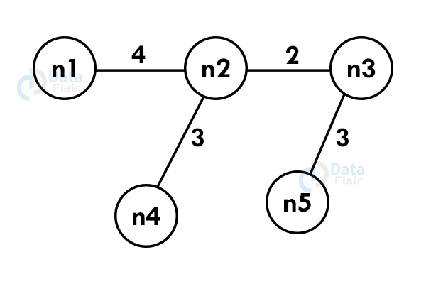
Step 4: Repeat the above steps until we include all the vertices and now you get the spanning tree.
6. Ford – Fulkerson algorithm
A greedy approach that calculates the maximum possible flow in a graph. A flow network has vertices and edges with a source(S) and a sink (T). All vertices can send and receive an equal amount of data but S can only send and T can only receive the data.
Basic terminologies used in the ford Fulkerson algorithm:
- Augmenting path: a path that is available in a flow network.
- Residual graph: flow network that has an additional possible flow.
- Residual capacity: capacity of edge after subtracting the flow from maximum capacity.
Algorithm:
- All flow in the edges is initialized to zero.
- If there is an augmenting path between source and sink, add the path to the flow.
- Update residual graph.
Let us analyze this algorithm for a system of pipes with a fixed maximum capacity.
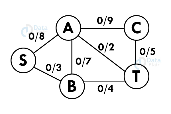
Step 1: Select a path from S to T. Here we select path S -> A -> T
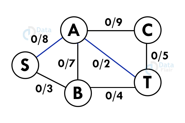
Step 2: Update the capacities. Here the minimum capacity is of edge A – T (2).
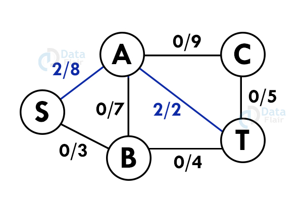
Step 3: Select another path. S – B – A – C – T
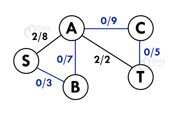
Step 4: Update the capacities again. Here minimum capacity is of the edge S – B.(3)
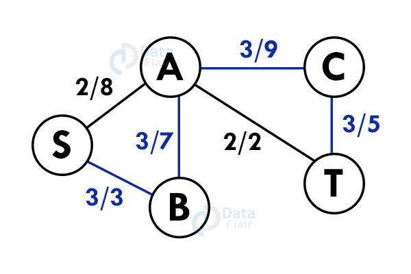
Add all the flows : 2+3 = 5. This is the maximum flow possible in the flow network.
7. Dijkstra’s algorithm
Dijkstra’s algorithm finds the shortest path between the two vertices but it might not include all the vertices of the graph. Dijkstra’s algorithm maintains the distance of every vertex.
For example:
Let’s start with a graph:
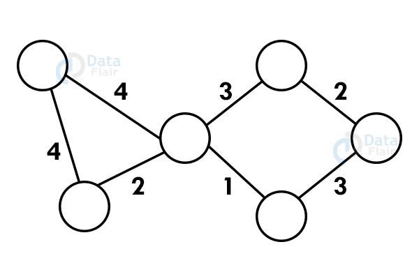
Step 1: Select any vertex as starting vertex.
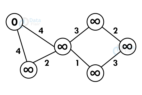
Step 2: Reach each immediate vertex and update the path distance.

Step 3: If the adjacent path is greater than the current path, don’t update the path value. Perform step 2 again.
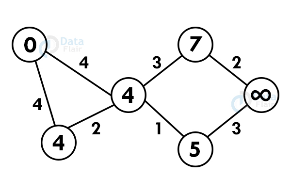
Step 4: Do not update the path of already visited nodes. To reach any unvisited node, select the path with the minimum path.
8. Prims algorithm
A greedy algorithm for minimum spanning tree that takes input in form of a graph and reserves the subset of edges of the graph which
- Forms a tree including every vertex
- Has minimum sum of weight among all the subtrees
Algorithm :
- Initialize the minimal spanning tree with any chosen vertex.
- Search for all the edges that connect the tree to new vertices, find the minimum from them, and add it to the tree. Perform the system recursively until you get a minimum spanning tree.
For example:
Let us consider the graph:-
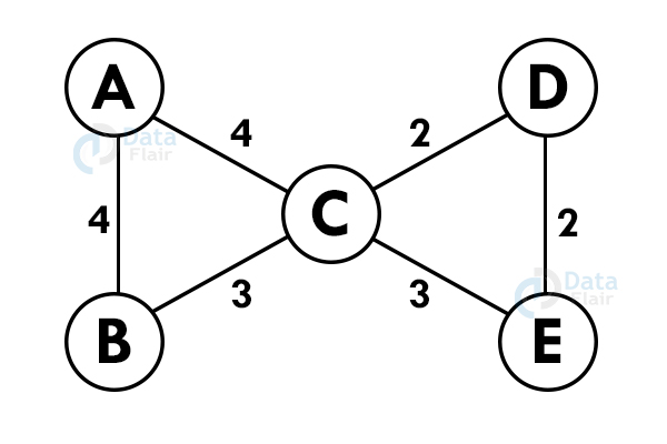
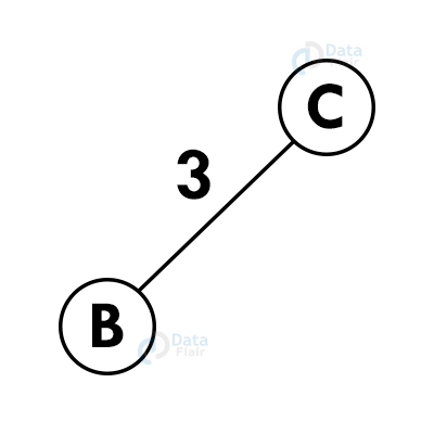
Step 1: Select any vertex at random.

Step 2: Select the shortest edge from this node and add it to the tree.
Step 3: Choose the nearest vertex which is not included yet.
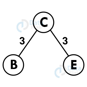
Step 4: Repeat the above steps recursively until we get the spanning tree.
Dynamic programming vs Greedy Algorithm
| Greedy | Dynamic |
| We choose which is best and then try to solve the problem arising after it. | We choose at each step, but it depends on the solution to subproblems. |
| More efficient at finding an optimal solution | Less efficient at finding an optimal solution |
| Example: fractional knapsack | Example: 0/1 knapsack |
| Might or might not get an optimal solution | Guaranteed optimal solution |
Conclusion
We have now seen in this article how greedy algorithms work and the properties required to design the greedy algorithms. We have seen a real-life example where the greedy algorithm fails to give the optimal solution. We have also seen some common real-world applications of algorithms.
Some applications and algorithms were also discussed in this article which has various large implementations in the real world. We will learn about these algorithms in detail in future articles.
You give me 15 seconds I promise you best tutorials
Please share your happy experience on Google


