Formulas and Calculations in MS-Excel
Expert-led Online Courses: Elevate Your Skills, Get ready for Future - Enroll Now!
MS-Excel is one of the software tools developed by Microsoft for easy computation, visual insights of the data using the features provided by the MS-Excel. In this tutorial of “What are Formulas and Calculations in MS-Excel?”, we’ll learn how to do basic calculations in MS Excel and what are the different ways to do a computation.
Performing calculations in MS-excel is quick and easy. The steps involved to do a calculation are very simple and there is nothing much to remember like you have to do in other coding languages.
Let us start with knowing what is a calculation?
In simple words, we could say calculation is a computation that starts with a ‘=’ symbol.
Basic operations in MS-Excel are:
- Addition
- Subtraction
- Multiplication
- Division
- Percent
- Power
- Square Root
A quick understanding of the basic operations in MS-Excel.
| Operation | Operator | Formula | Description |
| Addition | + | =A1+A2 =sum(start cell:end cell) | Summing of two values in the cells A1 and A2. |
| Subtraction | – | =A1-A2 | Subtraction of the value in the cell A2 from A1. |
| Multiplication | * | =A1*A2 | Product of two values in the cells A1 and A2. |
| Division | / | =A1/A2 | Dividing the value of cell A1 by the value in cell A2. |
| Percent | % | =A1*A2% | To find A2% of the number in the cell A1. |
| Power | ^ | =A1^A2 | Raising of the value in A1 by the power of A2. |
| Square Root | SQRT() | =sqrt(cell) | To find the square root of that particular cell. |
1. Addition in MS Excel
Now, let’s look at the ways in adding two or more values in a spreadsheet.
Steps to follow while summing up the values in the cells:
Step-1: You can just write the formula in the desired cell.
Step-2: Press ENTER.
For Example, You wanted to add the values of A2…A6 cell and see the result in D2 cell.
Hence, write =A2+A3+A4+A5+A6 in D2.
After writing it, once you press ENTER, the result appears as below.
The above method consumes much of the time if we have more data. To make it simpler and quicker, we can follow the SUM function method to calculate the sum in the spreadsheet.
To do so, follow the below steps:
Step – 1: Place the cursor on the desired cell.
Step – 2: Write the formula using the function “=sum(start cell:end cell)”.
Tip: When you don’t have the idea from where it has to start and end, then, just click and drag on the data to which the computation should apply.
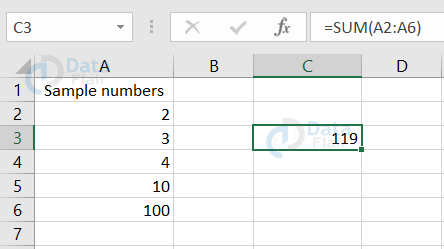
Note: Here the start cell mentions the first cell value of the sum computation. The end cell mentions the last cell value involved in the summation.
From the sample, we can see that C3 is the desired cell. It contains the sum from A2 to A6. Hence, we can say that the start cell here is A2 and the end cell is A6.
The above method is one of the most common methods to add multiple cells in a spreadsheet. Adding two or more cells is one of the basic operations performed in MS-Excel.
2. Subtraction in MS Excel
Next, let’s have a look at how to find the difference between the two numbers.
Another interesting fact in MS-Excel is that the operations are all similar. It does not have many changes in the steps. All that matters is that you have to provide the appropriate symbol for the calculation you are computing. Finally, you’ll get the desired result.
Now, let’s find the difference between two cells in a spreadsheet. To find the difference, follow the below steps:
Step-1: Write the formula in the desired cell.
Step-2: Press ENTER.
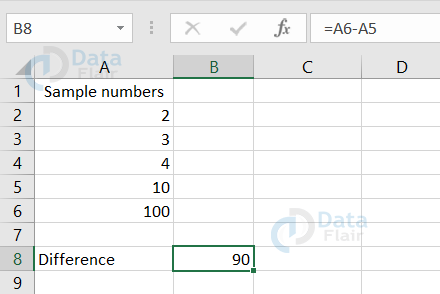
From the above sample, we can see that the difference between A6 and A5 in B8 using the formula“=A6-A5”.
3. Multiplication & Division in MS Excel
Further, we’ll look into the calculation of multiplication and division in the spreadsheet. To do so, follow the steps provided below:
Step-1: Write the formula in the desired cell.
Step-2: Press ENTER.
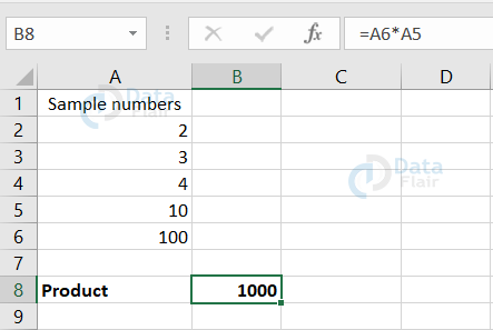
From the above sample, we can see that B8 contains the product value of A5 and A6 using the formula “=A6*A5”.
You have to follow the same steps to do division also.
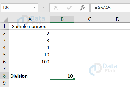
From the above sample, we can see that B8 contains the value of A6 divided by A5.
4. Average in MS Excel
Now, let’s have a look at how to calculate the average of the cells specified. To calculate the average, follow the below steps.
Step – 1: Choose the desired cell where you want to calculate the average.
Step – 2: Write the formula ‘=average(start cell : end cell).
Note: If you don’t know the start cell and the end cell, then just drag the cells by keeping the cursor inside the parentheses().
Step – 3: Press ENTER.
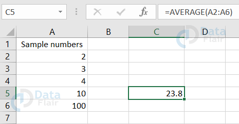
In the above sample, the C5 cell holds the average of A2…A6.
5. Percent in MS Excel
Next, we will see how to calculate the percent values in MS-Excel. To calculate the percent values, follow the below steps:
Step -1: Choose the cell in which the percent value should appear.
Step-2: Write the formula =cell number * x%
Note: Here, x is the percentage value. The x value can be directly entered or it can also be a cell number.
Step – 3: Press ENTER.
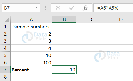
From the sample, we can see that B7 holds the 10% percent value of A6. The percent value is 10 here and that value is also taken as a cell itself. It is in cell A5.
6. Power in MS Excel
Next, let’s look at how to find the power of a number in MS-Excel. The same steps apply here also. Only the symbol keeps changing.
To find the power of a number, we’ll use the notation “^” between the numbers.
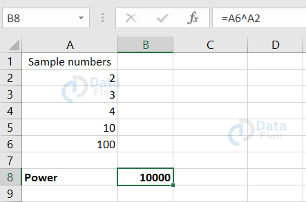
From the sample, we can see that B8 contains the power of the desired cell.
The base in this sample is A6 and the power is A2. Hence, we write it as A6^A2 in B8.
7. Nth Root in MS Excel
We can also find the nth root of a cell using the formula of= ^(1/n). Here n = root to find.
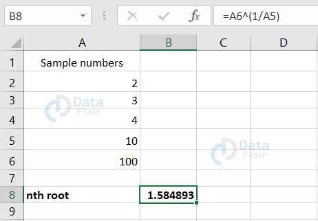
In the above sample, we have found the 1/nth root of A6 in the cell B8. Here n=10 and even that value is taken from cell A5.
8. Square Root in MS Excel
Now, Let’s calculate the square root of a number. To calculate the square root, we’ll be using the function SQRT().
Step -1: Click on the cell in which square root of a number should appear.
Step -2: Write the function i.e., =sqrt(cell) or sqrt(number).
Step-3: Press ENTER.
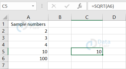
In the sample, we can see that the C5 cell holds the square root of the cell A6. Let us also have a look at how to perform the Trim function:
TRIM:
Trim is a function that helps in removing the extra spaces in a cell. It works only on a single cell at a time. To apply the function ‘Trim()’, follow the steps as below:
1: Choose a cell where the trimmed data should appear.
2: Write the function as ‘=TRIM(cell number)’
3: Press Enter.
Let’s look at a sample of how it works:
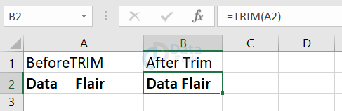
From the sample, the elimination of extra space in the cell A2 has taken place and the result is observed in cell B2.
9. Concatenation in MS Excel
Concatenation is the merging of two or more cell values in a single cell. Usually, “&” is known as the concatenation operator. To do this, we can use the formula ‘=cell1 & cell2 & cell3 & …….&cell n’
Note: If we want space between the cells then re-write the formula as ‘=cell1&” “&cell2&” …“&cell n’. The space character(“ ”) represents the space between the concat words. To apply concatenation in your MS-Excel, follow the below steps:
1: Choose the cell where the concatenation should take place.
2: Write the formula
3: Press ENTER.
Let’s look at a sample of how concatenation works.
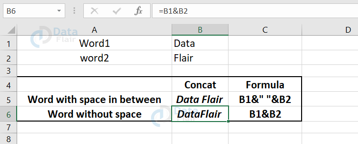
Using the formula, we have concatenated the words in B1 and B2. If we want to add space in between the words, then add an ampersand with a blank space in between the quotation(& “ “&).
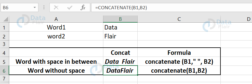
There is also another way to concatenate the values in the cell and that is by using CONCATENATE function.
To concatenate using the function, follow the below steps:
Step – 1: Choose the cell where the concatenation should take place.
Step – 2: Write the function formula ‘=concatenate(cell value, cell value,..cell value).
Note: If you want to add space between the words then write the function as ‘=concatenate(cell value, “ ”, cell value, “ ” ,…cell value)’.
Step – 3: Press ENTER.
Have a look at the image below for a clear understanding:
10. Comparisons in MS Excel
Using logical operators, we can perform the comparisons. If the condition satisfies, then the result appears either as true or false.
The logical operators are:
- = (Equal to)
Checks whether the data on the right and the left-hand side are equal.
- < (Lesser than)
Checks whether the data on the left-hand side is lesser than the right-hand side data value.
- > (Greater Than)
Checks whether the data on the left-hand side is greater than the right-hand side data value.
- <= (Lesser than or equal to)
Checks whether the data on the left-hand side is lesser than or equal to the right-hand side data.
- >= (Greater than or Equal to)
Checks whether the data on the left-hand side is greater than or equal to right-hand side data.
Let’s see how this works on excel with a sample.
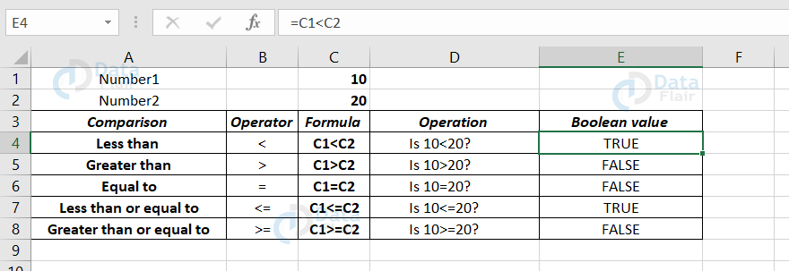
In the sample, we have taken the values 10 & 20 in the cells c1 & c2.
Using the logical operators, we have formed the table accordingly. If the condition satisfies, then it results as true in the cell or else it results as false.
If you want to perform more than one calculation in a cell, then, there comes the role of the precedence table.
11. Precedence Table in MS Excel
When there are more than two computations in a formula of a cell, there comes the role of a precedence table. The order of precedence plays a role while computing a complex formula.
| Precedence Order | Operator | Operation |
| 1 | – | Negation |
| 2 | % | Percent |
| 3 | ^ | Power |
| 4 | * , / | Multiplication & Division(In these both operations, whichever comes first will take the precedence.) |
| 5 | +,- | Addition & Subtraction(In these both operations, whichever comes first will take the precedence.) |
| 6 | & | Concatenation |
| 7 | >, <, >=, <=, = | Comparison |
Changing the order of the performance in MS Excel
If we want to change the order of performance, then those values can be given in the brackets. If the values are provided in the parentheses then those values will be computed first.
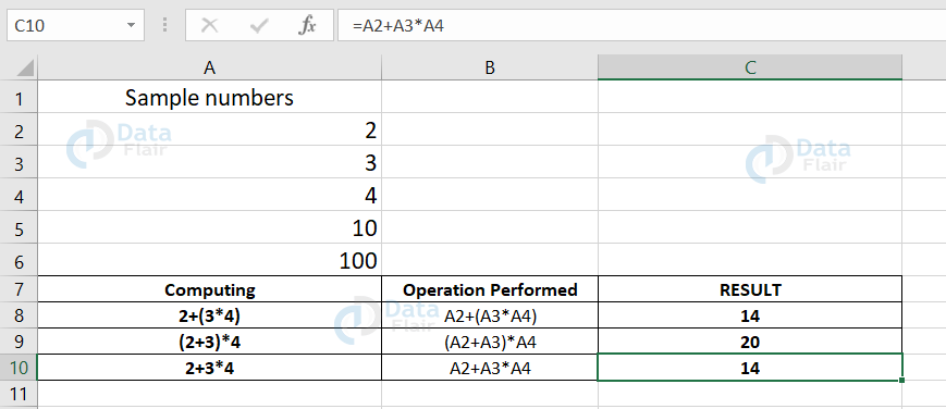
From the sample, we can understand that the parentheses are computed first and then the other value.
In cell c8, the products of A3, A4 are found and then they are added up with A2.
In cell C9, the sum of A2, A3 are found and then they are multiplied by A4.
As In cell C10, there were no parentheses found and so it has followed the precedence order. In between the multiplication and addition, the multiplication has higher precedence and so the values in the A3, A4 cells are multiplied first. And then, they are added with the value in cell A2.
Alternative ways to perform calculations in MS Excel
There are also other ways to perform calculations in MS- excel. They are:
- Using the AutoSum Function
- Through the Insert Function
- Using the Formulae from the group
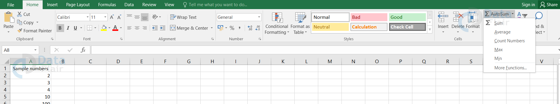
1. Using the AutoSum function in MS Excel
To use the autosum function for calculations, follow the below steps:
- Click on the Home tab.
- Go to the AutoSum option and click on the dropdown menu to choose the required function.
- Click on the function and start performing the calculation.
Now, Let’s have a glance at the functions in autosum and what they perform:
| Function | Formula | Syntax | Description |
| Sum | Sum() | =sum(start cell: end cell) | It calculates the sum of the cells. |
| Average | Average() | =Average(start cell:end cell) | It calculates the average of the cells. |
| Count Numbers | Count() | =count(start cell: end cell) | It counts the total number of cells. |
| Max | Max() | =Max(Start cell: End cell) | It picks the cell which has maximum value in it. |
| Min | Min() | =Min(Start cell: End cell) | It picks the cell which has minimum value in it. |
Sum using AutoSum Function:
To calculate the sum using autosum function, follow the below steps:
STEP-1: Click on the home tab and choose the autosum function.
STEP-2: Click on the drop-down option and choose sum.
STEP-3: Once the function appears, then just drag to which all cells the function should apply.
STEP-4: Press ENTER.
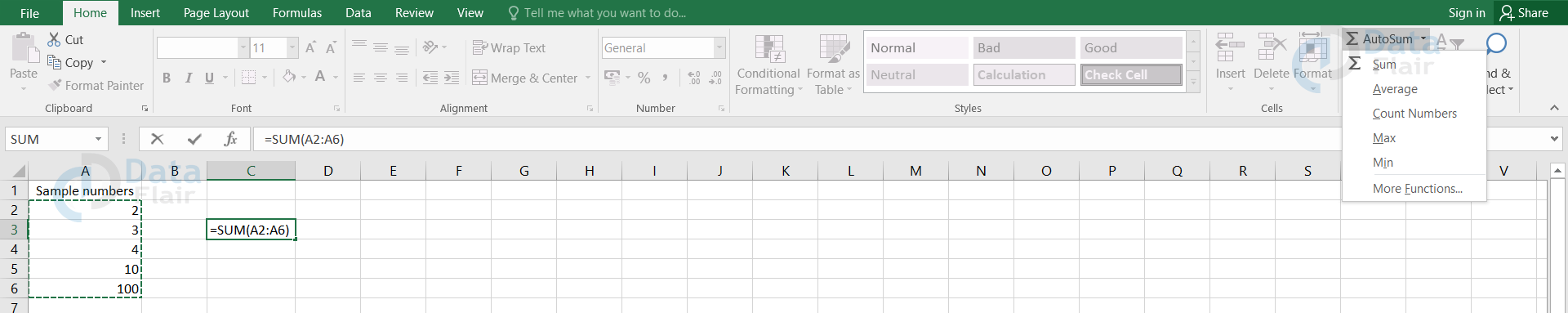
In the above sample, C3 holds the sum value using the sum function in AutoSum.
Average using AutoSum Function:
If you want to calculate the average using autosum, follow the steps as below:
Step -1: Choose the cell.
Step -2: Click on the home tab and navigate to the autosum.
Step-3: Click on the drop-down option in autosum. Choose average function.
Step -4: Drag the cells to which the function should apply.
Step-5: Then, press enter.
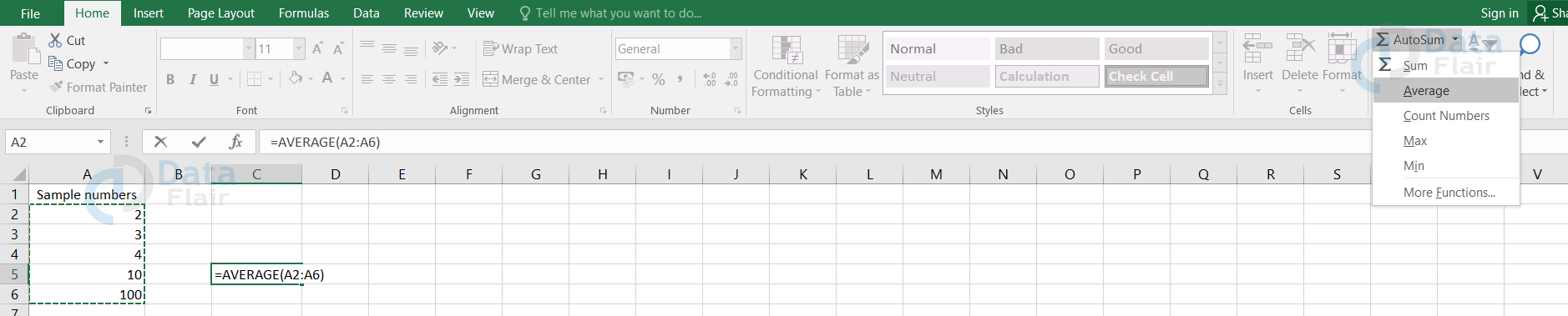
From the sample, we can see that C5 holds the average value of A2 to A6 using the average function in AutoSum.
Max, Min, and Count Numbers Functions using AutoSum:
Let’s have a quick look at how the max, min, and count numbers functions work.
To compute these above functions, the steps to follow will be the same. But make sure you choose the appropriate function before computing.
Below are the steps to follow to use an autosum function:
Step -1: Choose the cell.
Step -2: Click on the home tab and navigate to the autosum.
Step-3: Click on the drop-down option in autosum. Choose the required function.
Step -4: Drag the cells to which the function should apply.
Step-5: Then, press enter.
Count Numbers:
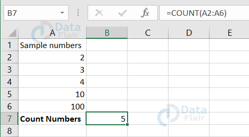
From the sample, we can see that the B7 cell holds the count of the number of values from A2 to A6 cells.
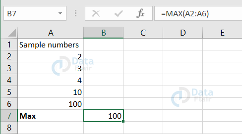
From the sample, we can observe that we have used the max function from autosum to show the maximum value from the list.
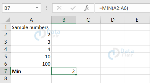
Here, we can observe that we have used the min function from autosum, to show the minimum value from the list
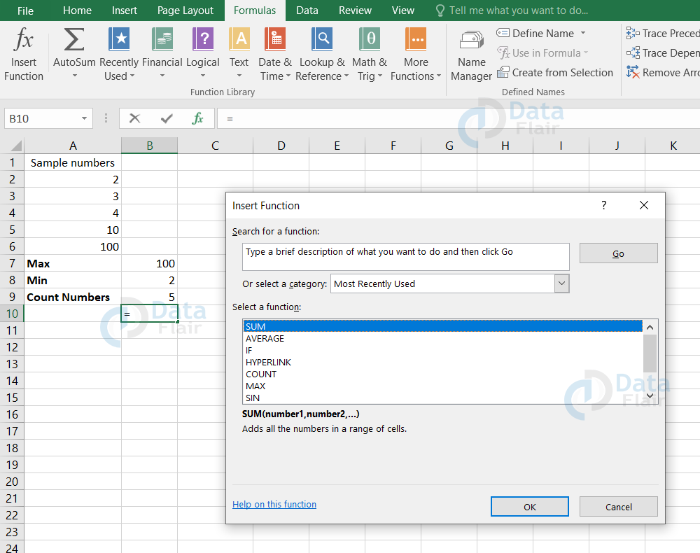
2. Using INSERT Function
One of the ways is to click on the Formulas tab and choose the Insert Function option.
Then a box appears with the list of functions.
If you don’t know the name of the function, then you can just search for the function in the place provided. And press GO.
Else, if you have an idea about the function name then just click on it and press OK.
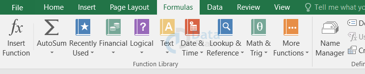
3. Using Formulae from the Group
The other way to perform a calculation is to choose the formula from the groups provided in the MS Excel.
Click on the Formulas tab and choose any of the groups relevant to your calculation.
The groups in MS-Excel are:
- Recently Used
- Financial
- Logical
- Text
- Date & Time
- Lookup & Reference
- Math & Trig
Each group contains the formulae related to their group name. The recently used group contains the formulae that are frequently used.
Summary
- From the above tutorial, we have understood that performing calculations in MS-Excel is quite simple and easy.
- The only thing that we have to remember is that we have to start an operation with an equal to (=) symbol if we are typing the function.
- We can also see what calculation we are performing in a cell by clicking on it. Formula bar helps you in viewing the calculation in a particular cell.
- There are many ways to perform calculations in MS Excel.
Your 15 seconds will encourage us to work even harder
Please share your happy experience on Google


