Excel Ribbon – Customize Ribbon in Excel

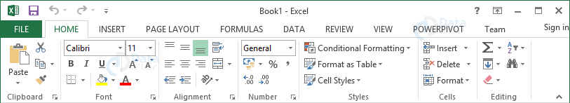
The row of tabs and icons at the top of the Excel window allows the user to access it quickly and use those commands for completing the task in the sheet. Ribbon is also considered as a complex toolbar. Excel 2007 version replaced the traditional toolbars in the previous version. Microsoft provided the ability to the users to personalize the ribbons from the version excel 2010.

Understanding the Ribbon in Excel

The ribbon in excel provides shortcuts to commands. The user uses the command to perform some actions in excel. An example of a command is saving a file, creating a new excel file etc.

Excel Ribbon components

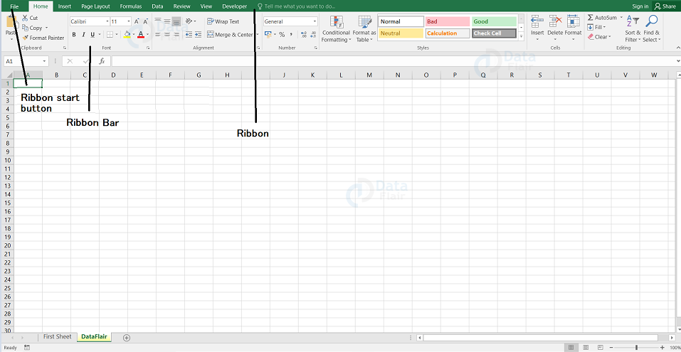
• Ribbon start button – It is used to access commands such as creating new documents, saving existing work, printing, etc.
• Ribbon – The tabs in the ribbon groups the similar commands together.
• Ribbon bar – The bars in the ribbon are used to group similar commands together. As an example, the font ribbon bar is used to change the font of the data.

There are four components in excel ribbon and they are tabs, groups, dialog launchers and command buttons.

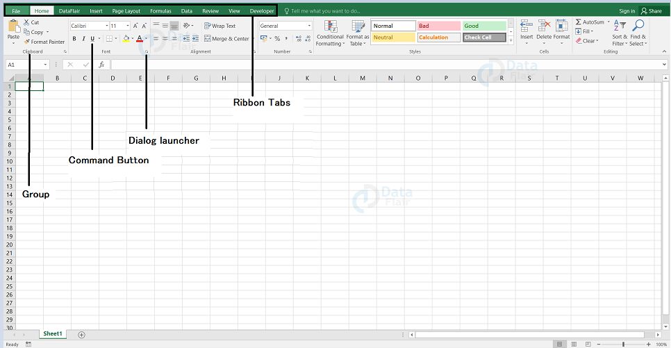
Ribbon Tab :

It contains multiple commands which are logically split into groups.

Ribbon Group:

It is a group of commands which are closely related and they are performed as a part of larger tasks.

Dialog Launcher :

It is a small arrow in the right corner of a group which brings up more related commands. It appears in the group’s right corner as a small icon.

Command Button:

It is the button a user clicks to perform a particular action.

Ribbon Tabs in Excel

There are few tabs available in the ribbons such as File, Home, Insert, Draw, Page layout, Formulas, Data, etc.

File:

It navigates the user to the backstage view which contains the information about the file and the excel options . It was introduced in the excel 2010 version as a replacement to the office button in excel 2007 and in earlier versions.

Home:

This tab contains the most frequently used commands in it.

Insert:

This tab adds different objects and charts in the spreadsheet such as Images, PivotTables, Charts, Symbols, Headers, etc.

Draw:

This tab appears based on the device the user uses. This lets the user draw with the digital pen, mouse. This tab is available from the version Excel 2013 and so on. But this tab is not visible like the developer tab by default.

Page Layout:

This tab provides the tool to the users to manage the worksheet appearance. This tab contains tools such as gridlines, page margins, object aligning, print area, etc.

Formulas:

This tab contains the tools for inserting the functions or formulas in the cell.

Data:

This tab provides the commands for managing the data even while connecting to the external data.

Review:

This tab provides the tools such as check spelling, add commands, protects worksheets and workbooks ,etc.

View:

This tab provides the commands for switching between the worksheet views and arranging the multiple windows etc.

Help:

This tab is available in the excel 2019 and office 365 versions. The help tab provides quick access to the help task pane and allows the user to contact Microsoft support.

Developer:

This tab provides access to the advanced features in excel such as macros, form controls and XML commands. This tab is not visible until the user enables it.

Contextual Ribbon Tabs:

The excel ribbon also has context-sensitive tabs which are also known as tool tabs. This shows up only when the users select a certain item such as tables, charts, shapes, etc.

For example, if the user selects a chart, then the design and format tab appears under the chart tools.

How to hide the Ribbon in Excel?

Minimizing the ribbon

The user can also minimize the ribbon by clicking on the symbol near the minimize symbol and then choose the auto-hide ribbon option.

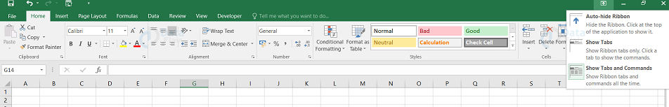
Auto-hide Ribbon:

Auto-hide shows the workbook in full-screen mode and once this option is chosen, it completely hides the Ribbon. To show the Ribbon again, click on the Expand Ribbon command at the top of the screen( three dots).

Show Tabs: When you click on this option, it hides all command groups when not in use, but the tab will remain clear. Simply click on the tab to maximize the ribbon.

Show Tabs and Commands: When you click on this option, it will maximize the Ribbon. All of the tabs and commands will be clear when this option is chosen.

Collapse the Ribbon in Excel

The user can collapse the ribbon to increase the size of the worksheet on the screen. When the user clicks on the collapse option, it hides the tabs and commands. To collapse the ribbon, right click anywhere on the ribbon and then select Collapse the Ribbon option.

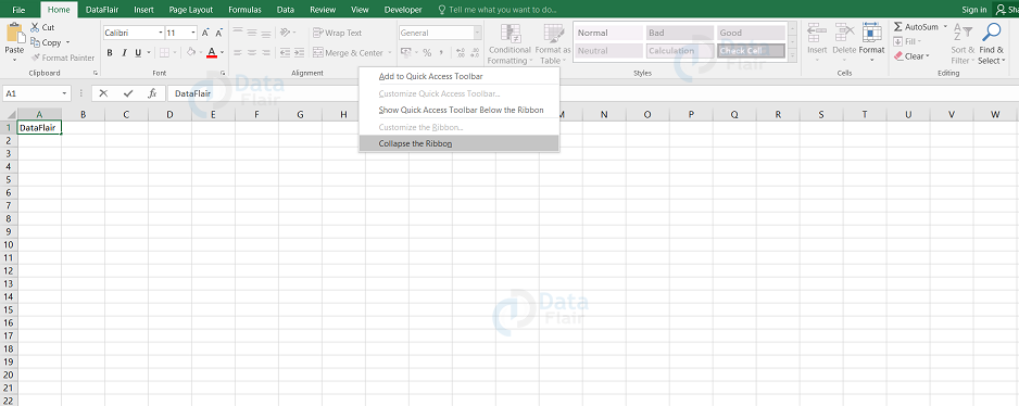
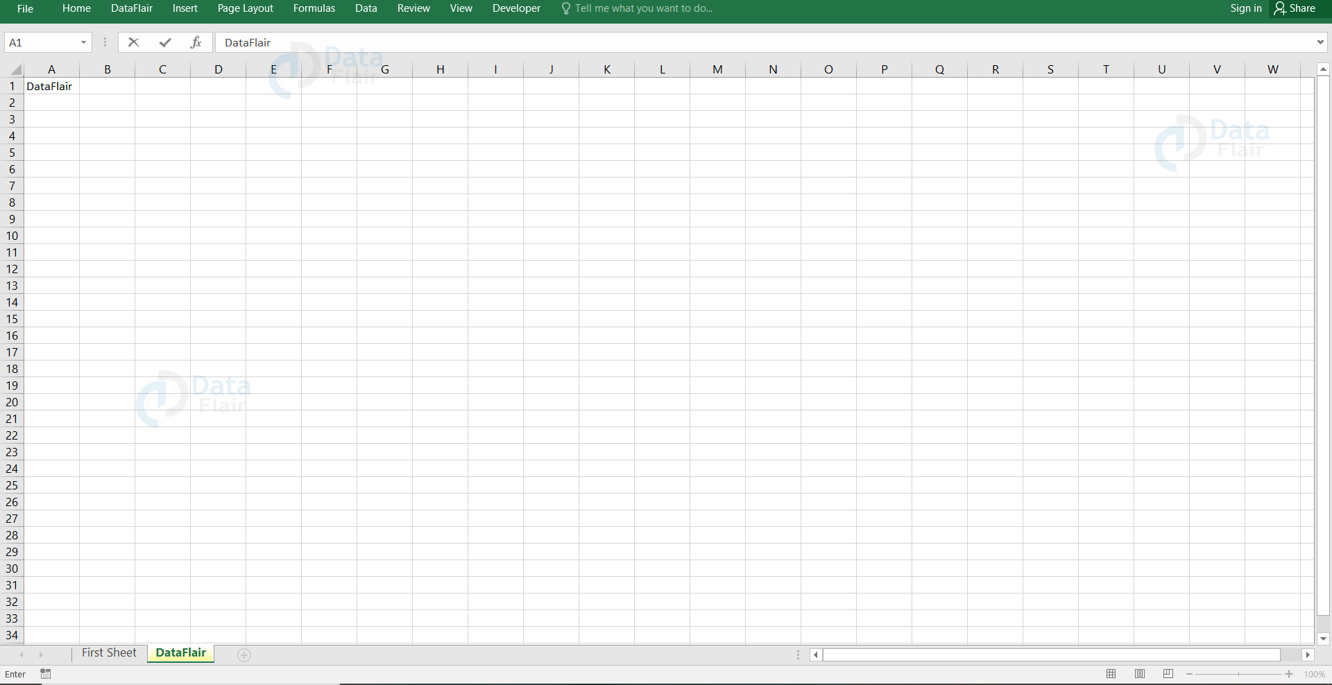
Note: When the user chooses the collapse option, the result appears as follows

Expand the Excel ribbon

If the user wants to make the ribbon be visible back again in the excel, then click on that small icon at the right side of the sheet and select show tabs and commands option.

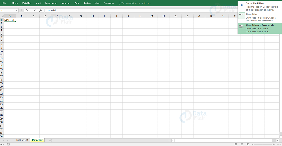
Note: When the user chooses the Show tabs and commands option, the result appears as follows: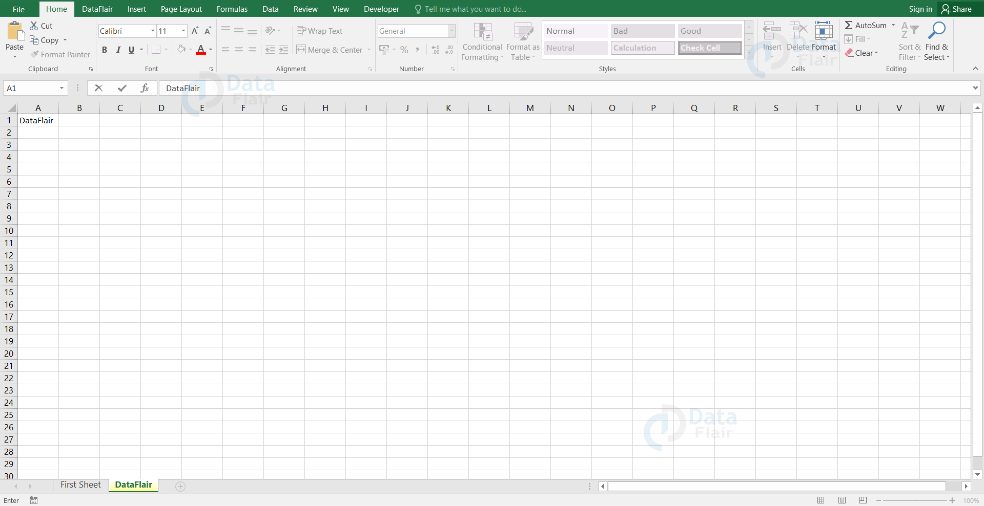

How to customize Excel ribbon?

If the user wishes to personalize the ribbon for their needs then they can also do that now. The entry point to most customizations is the Customize Ribbon window under the Excel Options. The shortest path to customize the ribbon is to right-click on the ribbon and select Customize the Ribbon from the menu.

Customizing the Ribbon in Excel:

You can also customize the ribbon and to do that, follow the steps:
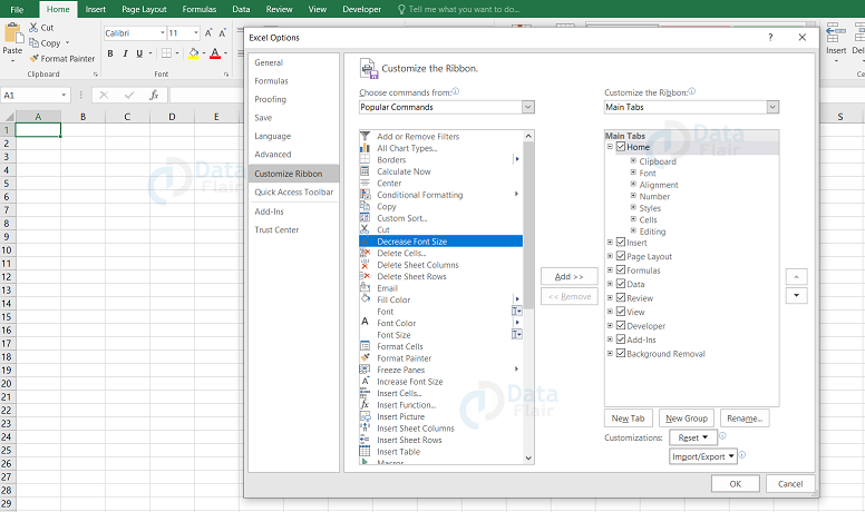
Step – 1: Click on the File tab
Step – 2: Choose options
Step- 3: Click on the customize the ribbon option from the left side of the panel.
Step – 4: Customize the ribbon by adding the required commands.
Step – 5: Once done, click on the ok button.

Adding custom tabs on the ribbon:

You can also customize the tabs on the ribbon. To do so, follow the steps:
Step – 1: Click on the file tab and choose options.
Step – 2: Select customize the ribbon option from the left side of the panel.
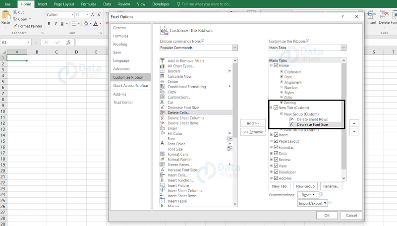
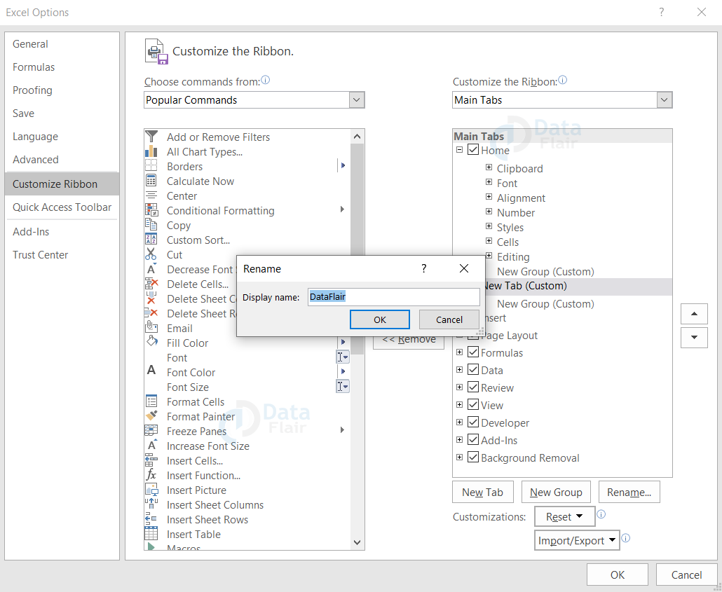
Step – 3: Click on the new tab button and the new tab appears in the list.
Step – 4: Right click on it and rename the tab.
Step – 5: Select the New Group (Custom) under the new tab.
Step – 6: Add commands to the ribbon bar.
Step – 7: Click on the ok button.

How to show the Developer tab in Excel?

The developer tab is an additional tab to the excel ribbon and this tab allows the user to access the advanced features such as Form controls, VBA Macros etc. The one disadvantage is that the Developer tab is hidden by default. But it’s very easy to enable it.

Developer Options

Step 1: To get the Developer Options tab, first we need to right click on the Home, click on the Customize the Ribbon button and that leads to a Dialog Box.

Step 2: From the Customize the Ribbon tab, check the Developer Options to enable the Developer tab and then click Ok.

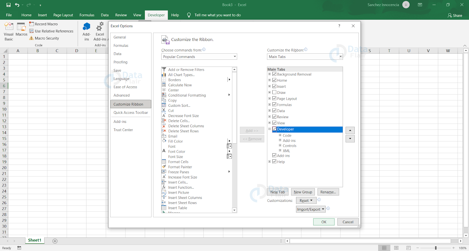
Step 3: Here, you find the Developer tab being enabled in the ribbon.

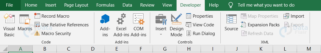
Note: To remove the developer tab from the sheet, follow the same steps but uncheck the box beside developer option and press ok.

Customization of Microsoft Excel Environment

The excel environment can be customized as per the requirement of the user. The user can change the colour theme, formulas and customizing the ribbon etc.

• Customization the ribbon
• Setting the colour theme
• Settings for formulas
• Proofing settings
• Save settings

Customization of Excel Ribbon

If the user wants to add some tabs that are missing or to remove some tab, follow the steps:

Step – 1: Click on the file tab.

Step – 2: Select options from the list.

Note: An Excel Options dialog window appears.

Step – 3: Choose the customize ribbon option from the panel.

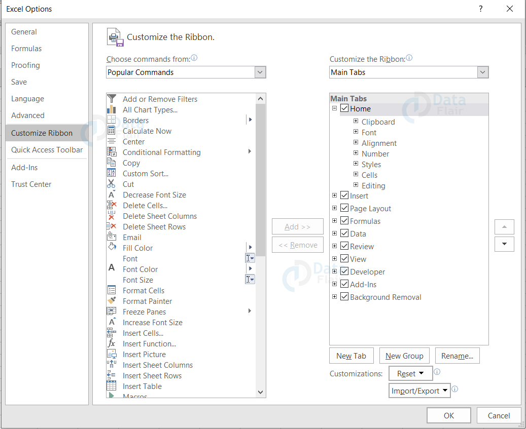
Step – 4: On the right-hand side, remove the check marks from the tabs that the user doesn’t require on the ribbon.

Step – 5: Click on the “OK” button.

Adding custom tabs to the ribbon in Excel

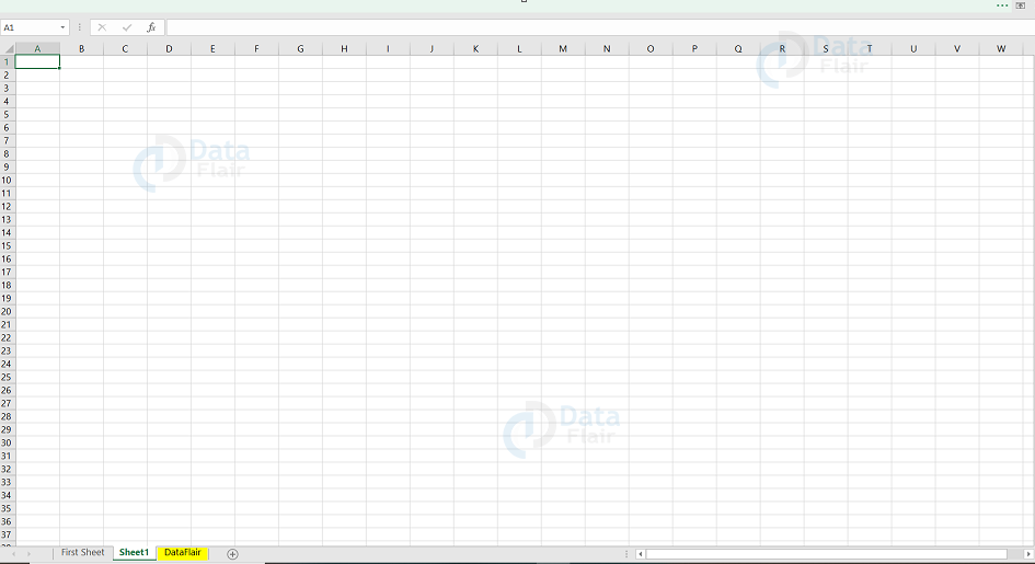
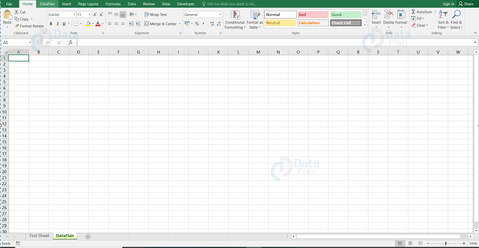
The user can also add their own tab, give it a custom name and assign commands as required. Let’s add a tab to the ribbon with the text DataFlair. To add custom tabs, follow the steps:

Step – 1: Click on the file tab.
Step – 2: Select options from the list.
Note: An Excel Options dialog window appears
Step – 3: Choose the customize ribbon option from the panel.
Step – 4: Click on the new tab button and rename it accordingly.
Step – 5: Add the commands required to the newly created tab.
Step – 6: Click on the ok button.

Your ribbon appears as follows:

Setting the color theme in Excel

To set the color theme for the Excel sheet, the user has to go to the Excel ribbon, and click on the File tab and choose the option command. It will open a dialog window. To set the colour theme, follow the steps:

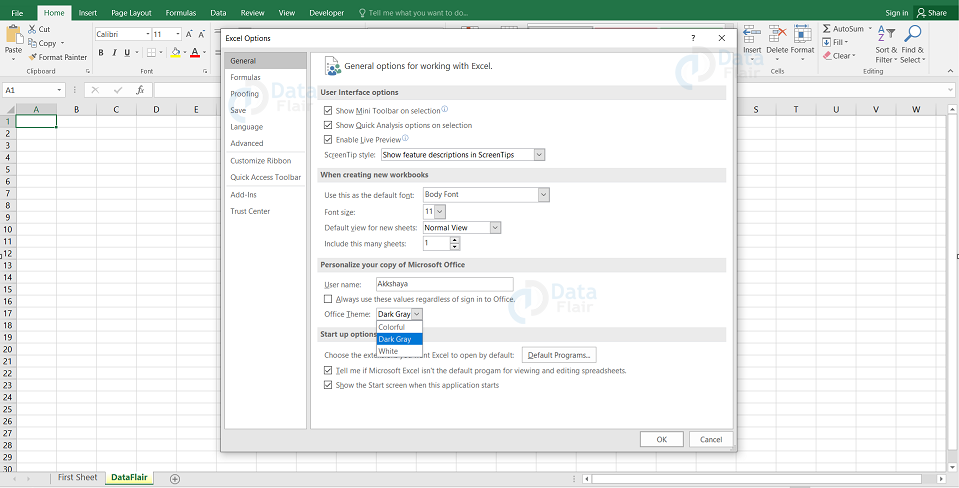
Step – 1: Go to the general tab from the panel.
Step – 2: Click on the colour scheme under General options.
Step – 3: Click on the drop-down list and select the colour which is required.
Step – 4: Click on the OK button.

Settings for Excel formulas

This option allows the user to define how Excel behaves when they are working with the formulas. The user can use it to autocomplete when entering formulas, change the cell referencing style etc.

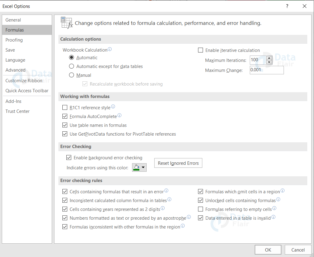
If the user wants to activate an option, click on the check box. If the user wants to deactivate an option, remove the mark from the checkbox. The user can use this option from the options dialog window and go to the formulas tab from the panel.

Excel Proof settings

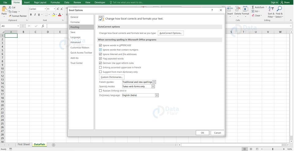
This proof setting helps the user to manipulate the entered text in the cell. It allows the settings options to check for the wrong spellings, suggestions from the dictionary, etc. The user can use this option from the options dialog window and go to the proofing tab from the panel.

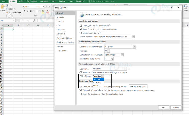
Color Theme Setting:

You can also set color theme for your excel and you can set it by following the steps:
Step – 1: Click on the file tab and choose general.
Step – 2: Go to the office theme and select the desired color from the drop down list.
Step – 3: Press ok.

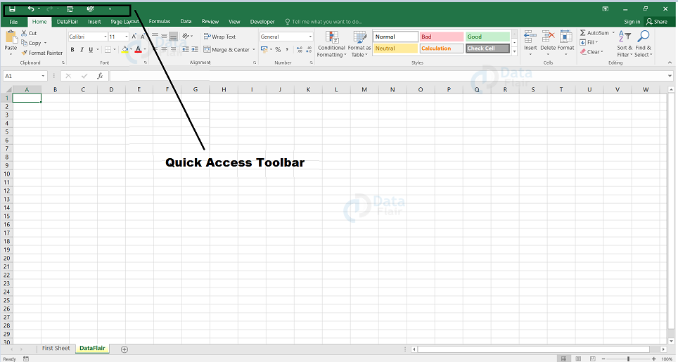
What is a Quick Access Toolbar?

The frequently used commands at the top of the application window are known as the quick access toolbar. These commands are accessed at any part of the application and it is not dependent on the ribbon tab which is opened.

The quick access toolbar is a drop-down menu containing a set of commands. It also includes an option to add the user’s own commands. There is no limit in the number of commands in the quick access toolbar and also the commands which are visible depending on the size of the window.

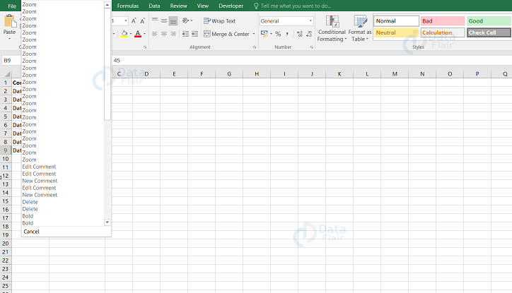
Undo Changes

Using the Undo command, the user can reverse the actions in MS Excel. To undo changes, follow the step:

• Click on the undo icon from the quick access toolbar.
• Or else press Ctrl+Z.

Note: The user can reverse nearly 100 past actions that are performed by executing undo more than once. The list of the actions appears when the user clicks on the arrow button. Click an item from the list to undo that particular action.

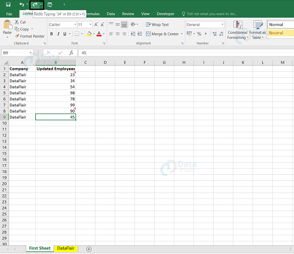
Redo Changes

The user can also reverse back the action by clicking on the Redo icon.
To Redo changes, follow the steps:

• Click on the redo icon from the quick access toolbar.
• Or else press Ctrl + Y.

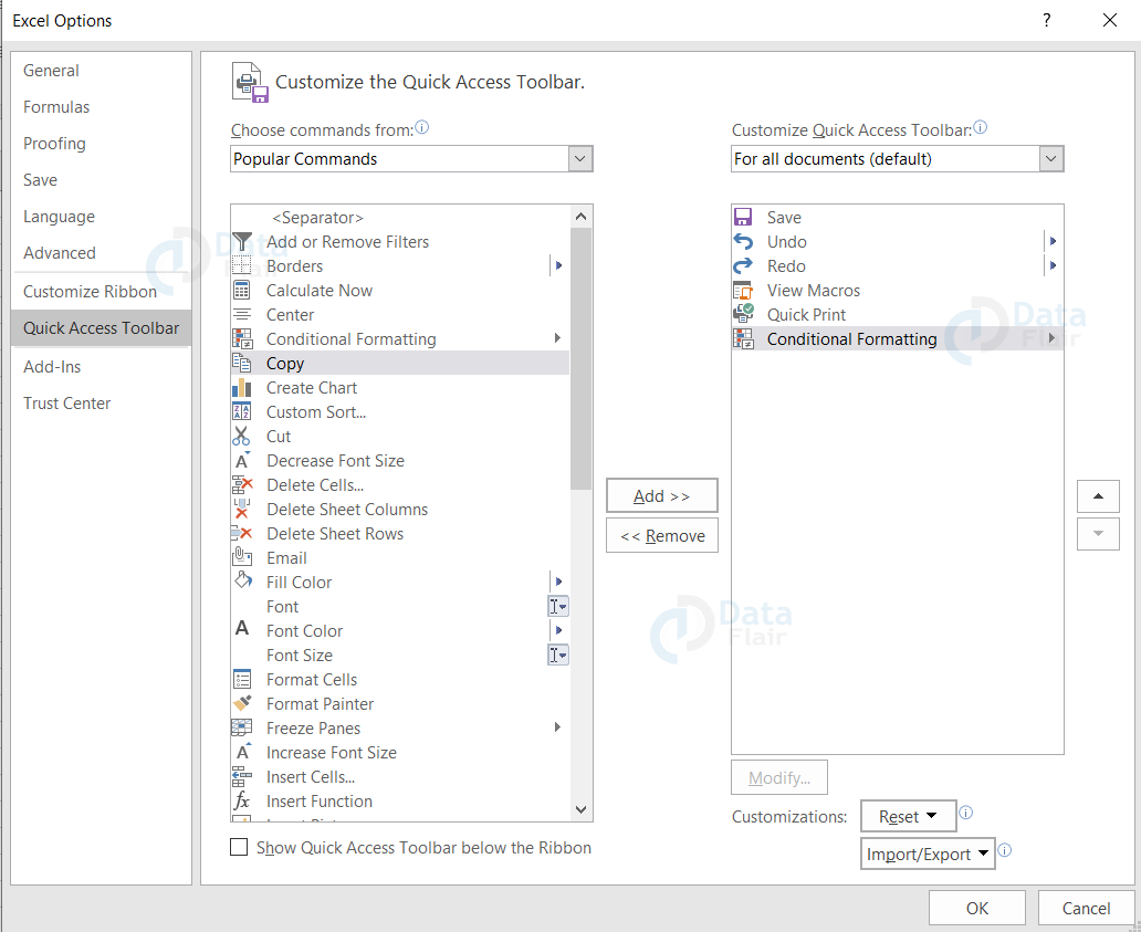
There are three ways to Customize the Quick Access Toolbar window

Method – 1: Click on the file tab, select options and go to the quick access toolbar. Add the required options to the quick access toolbar and finally press the ok button.

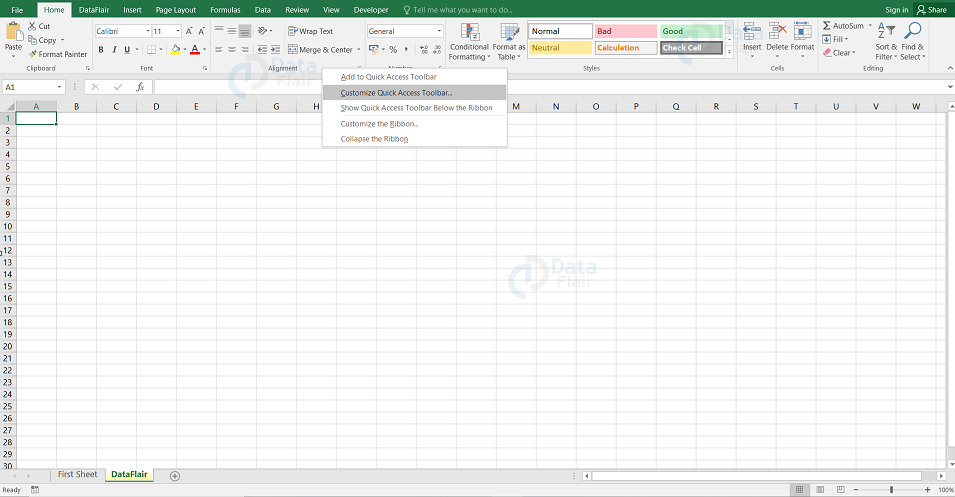
Method – 2: Place the cursor anywhere on the ribbon, right click and select the customize quick access toolbar.

Method – 3: Click on the down arrow at the top of the excel sheet. The down arrow is the quick access toolbar icon. Choose More Commands from the menu.

Note: The dialog window appears and the user can add, remove and reorder the quick access toolbar commands.

How to add a command button to Quick Access Toolbar?

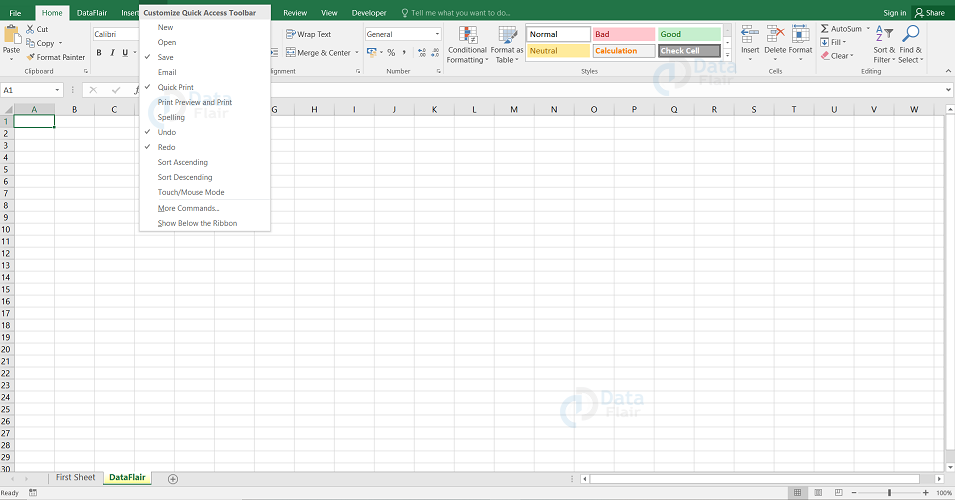
To enable command from the quick access toolbar, follow the steps:

Step 1: Click on the Customize Quick Access Toolbar button from the excel file.

Step 2: Enable the command that you want to see in the quick access toolbar menu.

For example: If the user wants to enable the spell check, select the spelling option from the list and immediately the button appears in the quick access toolbar.

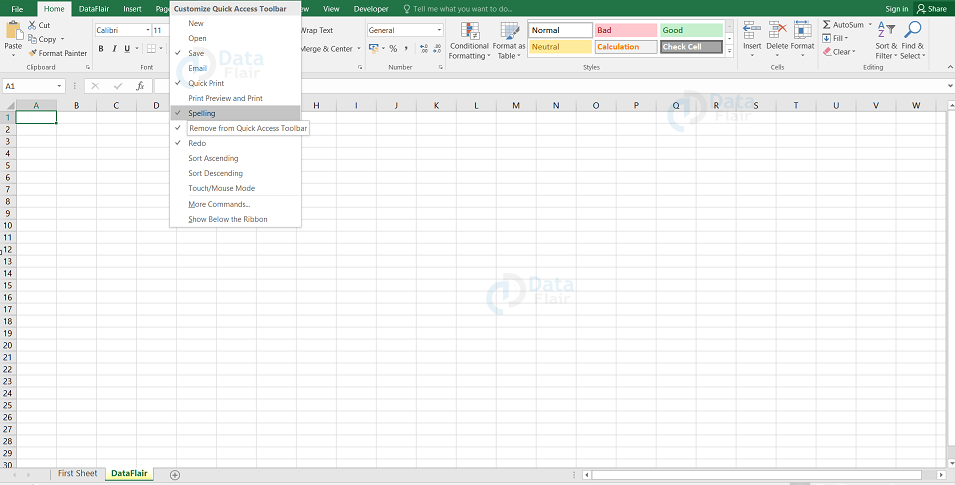
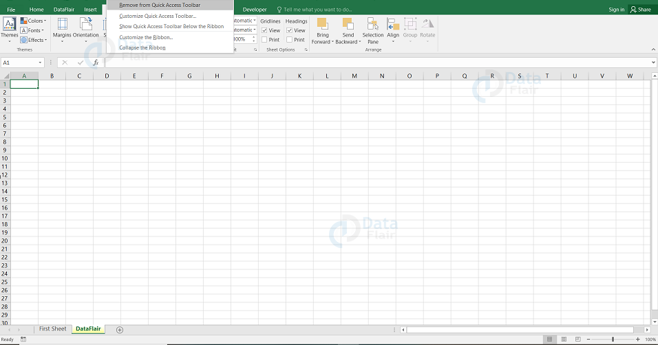
How to remove a command from Quick Access Toolbar?

To remove a command from the Quick Access Toolbar, right-click on the toolbar and select Remove from Quick Access Toolbar from the menu:

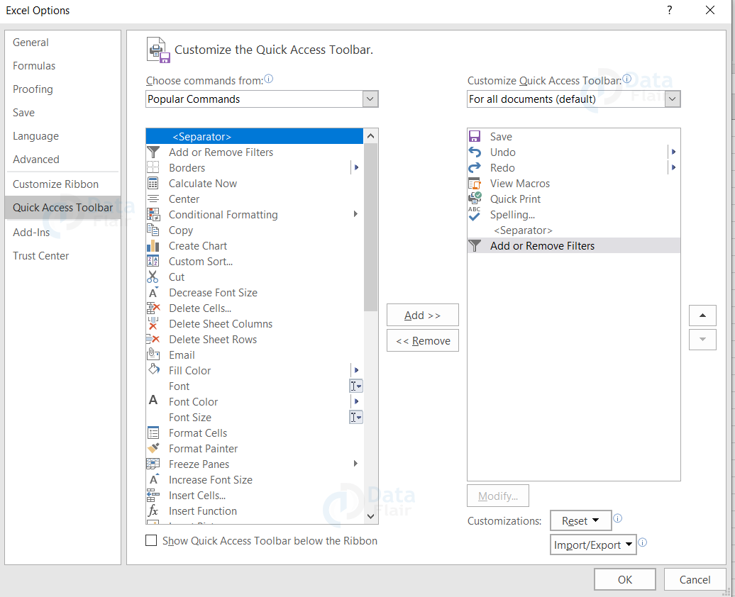
How to rearrange commands on Quick Access Toolbar?

To rearrange commands, follow the steps:

Step 1: Right-click on the toolbar and select the customize Quick Access Toolbar from the menu.

Step 2: Select the command that the user wants to move and click the Move Up or Move Down arrow.

For example, the user wants to move the spelling above the quick print, select it and click on the up arrow.

Step 3: Press the OK button.

Group commands on Quick Access Toolbar

If there are alot of commands, the user may want to sub-divide the functions into logical groups.
Though the Quick Access Toolbar does not allow creating groups like on the Excel ribbon, the user can group commands by adding a separate group tab. To add a group commands on Quick Access Toolbar, follow the steps:

Step 1: Right-click on the toolbar and select the customize Quick Access Toolbar from the menu.

Step 2: Choose commands in the dialog window and select popular commands.

Step 3: Choose the <Separator> option and click on the Add.

Step 4: Press on the Move Up or Move Down arrow to position the separator.

Step 5: Press the OK button.

Customizing the Quick Access Toolbar only for the current workbook

When the user customizes the quick access toolbar in excel, it is customized for all the workbooks by default. But if the user likes to make certain customizations for one particular workbook then select the current workbook from the customize quick access toolbar and then add the commands as required.

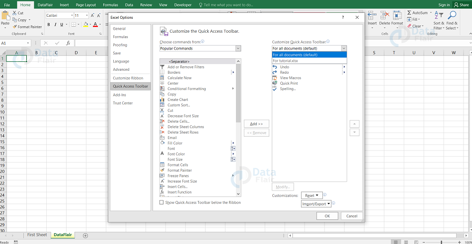
Note: The customizations made for the worksheet does not replace the other quick access toolbar commands. The customized commands are added to it.

How to move the Quick Access Toolbar below or above the ribbon?

Quick Access Toolbar is situated at the top of the excel window and it is the default location of it. If the user finds it comfortable to have the ribbon below, then they can move it.

To move the Quick Access Toolbar below, follow the steps

Step 1: Click on the Customize Quick Access Toolbar button from the ribbon.

Step 2: Select the show below the ribbon option.

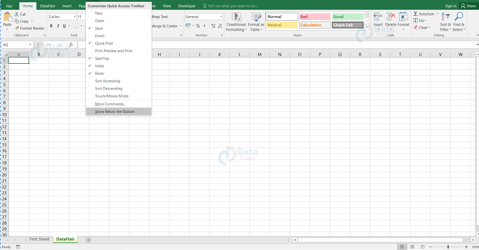
Note: To get the Quick Access Toolbar back to the previous location, click on the Customize Quick Access Toolbar button and then choose the Show Above the Ribbon option from the menu.

How to reset the Quick Access Toolbar to the default settings?

To reset the Quick Access Toolbar to the default settings, follow the steps:

Step 1: Right-click on the toolbar and select the customize Quick Access Toolbar from the menu.

Step 2: Click on the Reset button and then choose Reset only Quick Access Toolbar.

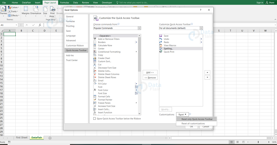
Step 3: Press the OK button.

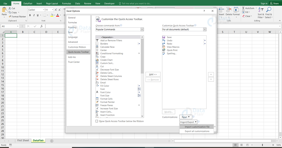
Export and import a custom Quick Access Toolbar

Microsoft Excel allows the user to save the Quick Access Toolbar and ribbon customizations into a file and this file can be imported later. This can help the user to keep the Excel interface looking the same on all the computers that the user uses as well as share the customizations with the other Excel users if they want.

• Export a customized Quick Access Toolbar:
  To export a customized Quick Access Toolbar, click on the Export all customizations under customizations and save the customizations file to a folder.
• Import a customized Quick Access Toolbar:
  Go to the Customize the Quick Access Toolbar window, choose Import/ Export and select the Import customization file from the option. The user can browse for the customizations file which was saved earlier.

Note:
The file that the user exports and imports also includes the ribbon customizations. There is no other way to export or import only the Quick Access Toolbar from the sheet.

When the user imports the customizations file to a system, all prior ribbon and the quick access toolbar customizations on that system are permanently lost. To be able to restore the current customizations, be sure to export it and save as a backup copy before importing any new customizations to the system.

Adding custom tabs to the ribbon in Excel

The user can also add their own tab, give it a custom name and assign commands as required. Let’s add a tab to the ribbon with the text DataFlair. To add custom tabs, follow the steps:

Step – 1: Click on the file tab.

Step – 2: Select options from the list.

Note: An Excel Options dialog window appears

Step – 3: Choose the customize ribbon option from the panel.

Step – 4: Click on the new tab button and rename it accordingly.

Step – 5: Add the commands required to the newly created tab.

Step – 6: Click on the ok button.

Your ribbon appears as follows:

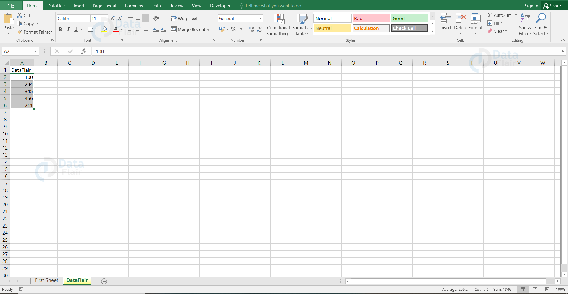
Excel Status Bar

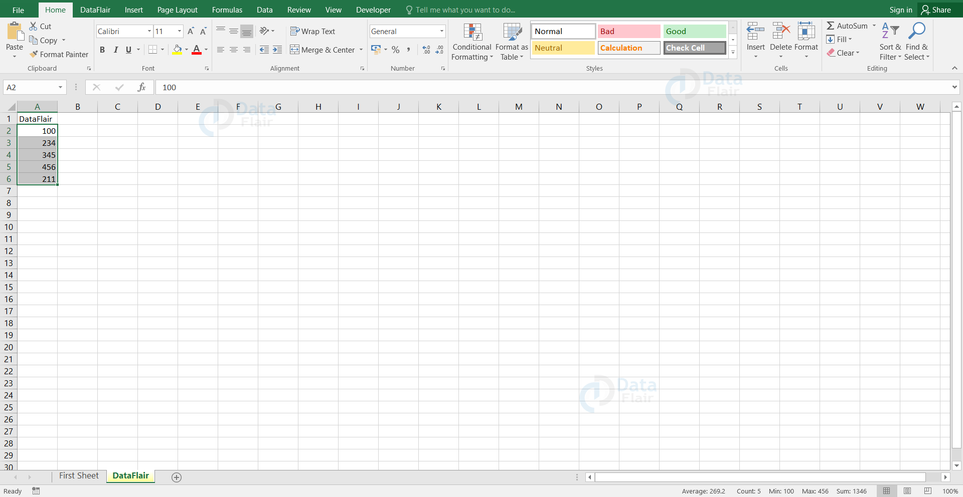
Status bar appears at the bottom of the sheet and it’s quite useful as it displays the average, count, sum, etc of the selected cell.

For a sample, let’s select the range A2:A6 in the sheet. Have a look at the status bar to see the average, count and sum of these cells.

Note: The status bar options are chosen by default. Right-click on the status bar to activate even more options to view in the status bar.

To view more options, follow the steps:

Step 1: Right-click on the status bar.

Step 2: Click on the required options. Here, we are choosing the maximum and minimum.

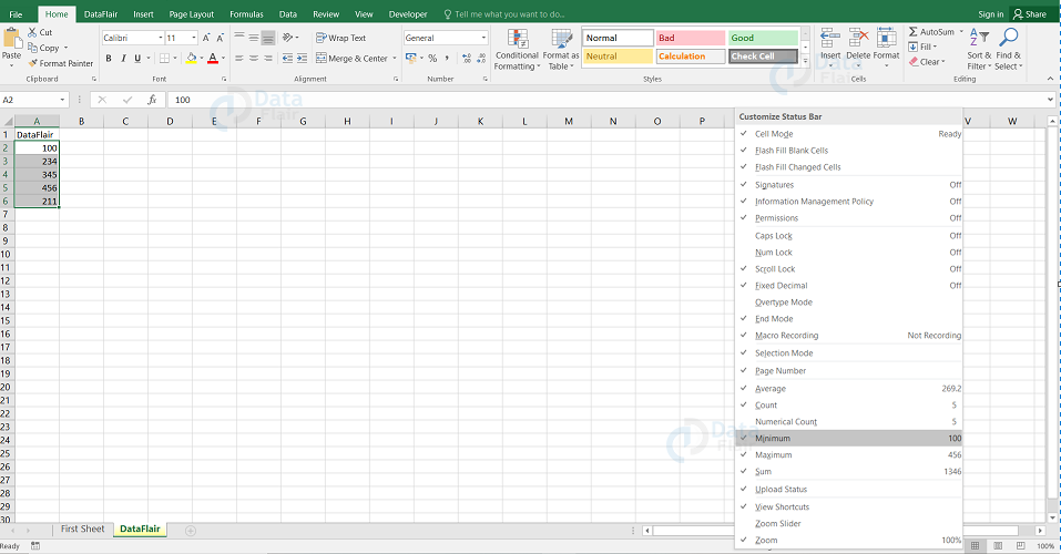
Note: Excel displays the minimum and maximum values also in the status bar.

Note: Excel uses the status bar in many situations and if the user does not want to view it, then they can hide it.

Checkbox in Excel

Inserting a checkbox and check mark in Excel is simple and easy. For example, let’s use a checkbox to create it in B2 cell.

Inserting a Checkbox

To insert a checkbox, follow the steps.

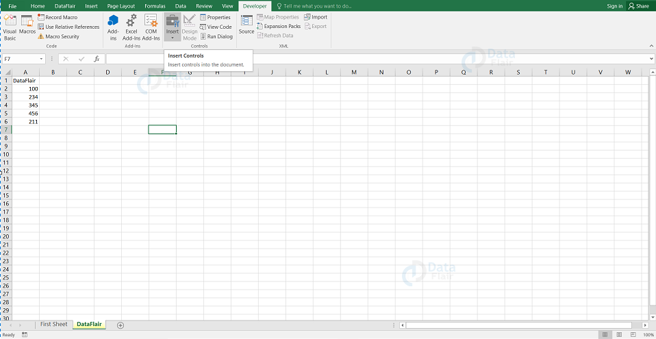
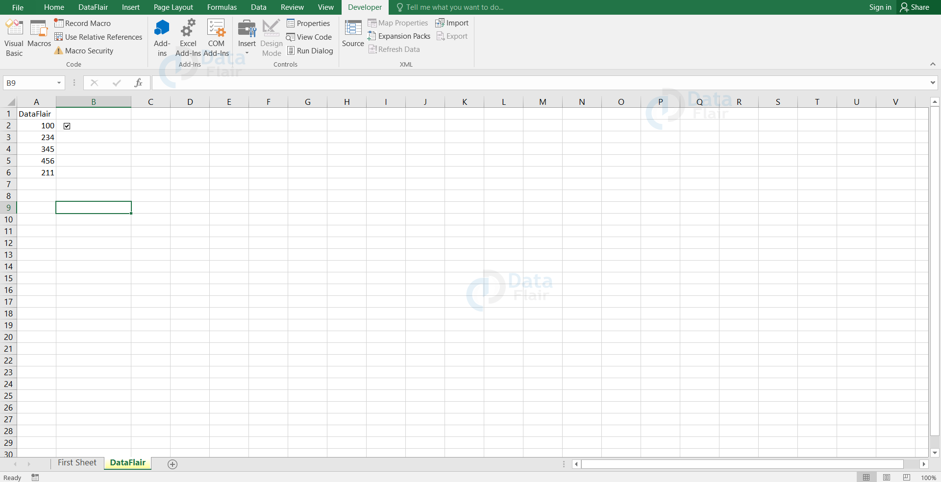
Step 1: Click on the developer tab and select the insert icon.

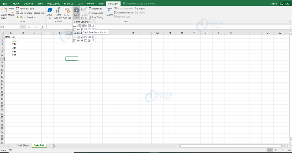
Step 2: Choose the Check Box from the Form Controls section.

Step 3: Place the cursor on the B2 cell and draw the checkbox.

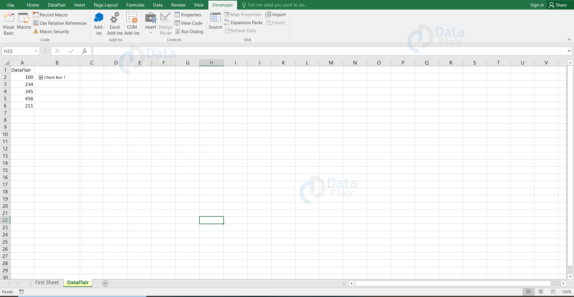
Step 4. To remove “Check Box 1”, right-click on the checkbox, select the text and delete it.

Link a Checkbox

To link a checkbox to a cell, follow the steps.

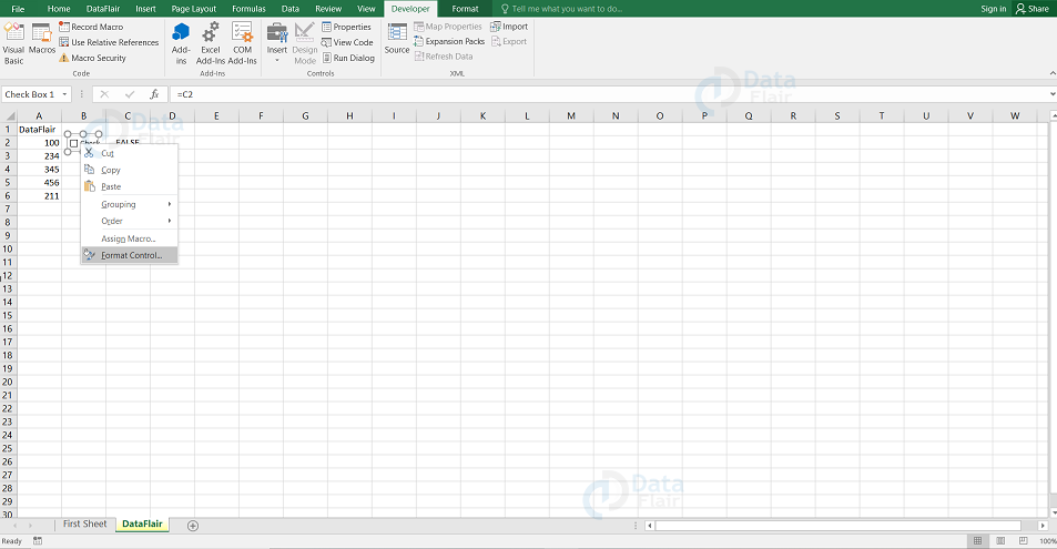
Step 1: Right-click on the checkbox and choose Format Control.

Step 2: Link the checkbox to the required cell. Here, it is C2.

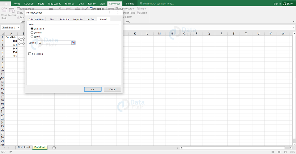
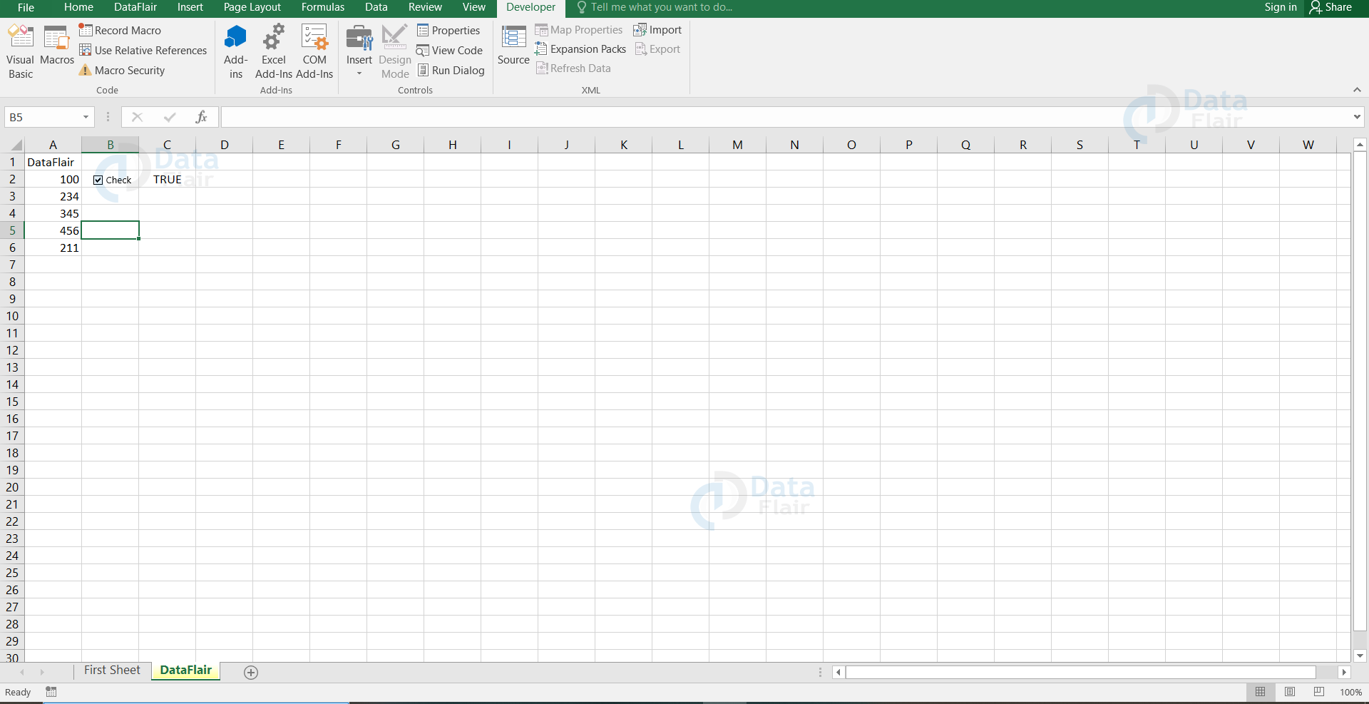
Note: Now, when the user clicks on the checkbox, the linked cell displays “True”

Step 3: Test the checkbox by marking on it.

Summary

The primary objective of the quick access toolbar is to store the frequently used commands in excel. The user can also customise the ribbon and quick access toolbar. The ribbon and quick access toolbar can be imported and exported from one system to another system also.