Excel formulas and functions
Job-ready Online Courses: Click, Learn, Succeed, Start Now!
Microsoft Excel helps in storing any type of data and the main advantage of using Excel is that there are various inbuilt functions available, which makes performing the calculations easy.
Microsoft Excel is one of the software used for data analysis. The expression which the user provides to calculate in an excel sheet is termed as formulas and the functions are already predefined in ms excel.
What is Excel Formula?
Excel formula helps the user to analyze the data easily. These help the user to calculate the values in the cells of the spreadsheet. They also save a lot of time and reduce the risk of making mistakes.
The instruction provided by the user to perform the calculations within the spreadsheet is called formulas.
The formula starts with an equal sign and then followed by the remaining part of the calculation formula. There is also another option available and in this method, the user can start a formula with either a plus (+) sign or minus (-) sign. Excel assumes that it is a formula, and once the user presses enter, the desired Excel formula’s result appears. If the user doesn’t type an equals sign first, then Excel assumes that the value is either a number or a text.
Some steps to follow for entering a formula into Excel.
1. Enter the formula in the desired cell.
2. To make excel understand that it is a formula, start it with an equal or plus or minus sign.
3. Complete the formula in the cell.
4. Press Enter to view the formula result.
Elements of Formulas in Excel
There can be any of the elements in the formula and they are:
a. Arithmetic operators in Excel
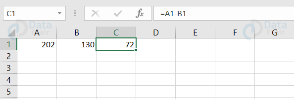
The operators such as + (for sum), – (for subtraction), * (for product) and / (for division)
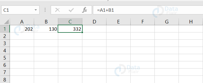
=A1+B1. This adds the values in cells A1 and B1.
b. Values or text
The string which can be numeric or text values.
=100*0.1. This multiplies 100 and 0.1 and this results in 10.
c. Cell references
This includes both named cells and ranges
=A1=B1. This compares the cell A1 with the cell B1. If the cell values are identical, then the formula returns true or else it returns false.
d. Worksheet functions
This includes the function from the worksheet such as countif, sum, average, etc.
=SUM(A1:A10). This adds the values in the range A1:A10.
Using Functions in Excel
When the user types the equal to (=) sign and an alphabet, the list of functions available with that alphabet will be listed.
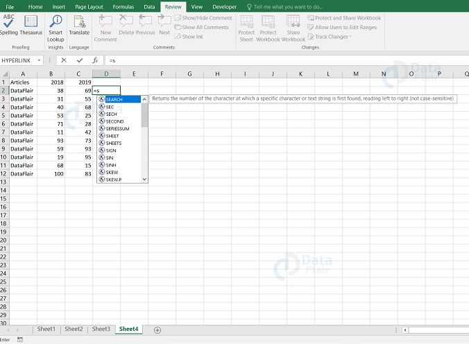
Here, the list of functions starting with S appears.
Function Arguments in Excel
The use of arguments varies in the functions. The arguments depend on what the function has to do. Each and every function uses the parentheses and the parentheses holds the list of arguments.
1. No arguments
These functions do not hold any argument between the parentheses. Example: TODAY()
2. One argument
These functions hold only one argument between the parentheses. Example: LOWER()
3. A fixed number of arguments
For a few functions, there are a fixed number of arguments to be provided and such functions are RANDBETWEEN(), IF() etc.
4. Infinite number of arguments
For few functions, there are no fixed number of arguments, we can keep on increasing the arguments and such functions are SUMIFS() etc.
5. Optional arguments
In few functions, there are optional arguments which means you can either provide them or you can leave it blank and the function considers the default value. EXAMPLE: VLOOKUP()
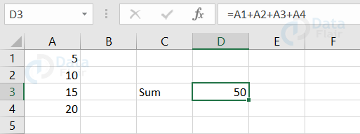
Formula Box in Excel
When the user wants to view the formula of a particular cell, then click on the cell and look at the formula box. Formula bar shows the contents of the current and allows the user to create and view formulas.

Errors in excel formulas
Sometimes, instead of getting desired Excel formulas results, the user may encounter an error in Excel. The two main types of Excel formulas errors are:
a. #value error
b. #name error
These errors occur mainly if the user types the invalid formula.
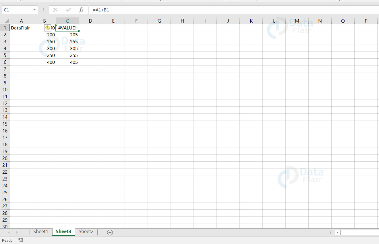
1. #VALUE Error in Excel
This error means that the formula entered is accepted but excel could not calculate a valid result from the formula.
For example Excel shows you a value error when the user tries to perform the arithmetic operation with numerical and non – numerical values.
Reasons for #VALUE Error
a. Performing arithmetic operations in the cells that contain a non-numerical value.
b. Error with the formula
c. Non-numerical values
This Excel formulas error is frequently encountered when the formula isn’t formatted correctly or contains other errors.
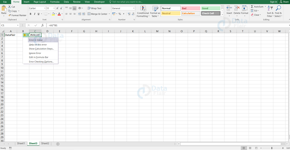
How to Correct #VALUE Error
Instead of using arithmetic operators, make use of the functions such as SUM, PRODUCT, or QUOTIENT, to perform an arithmetic operation rather than using arithmetic operators.
Make sure that the adding cell does not contain a non-numerical value.
To solve the error, click on the warning symbol provided at the side of the cell.
2. #NAME Error in Excel
This error occurs when excel doesn’t recognize text in the formula. When the user enters a wrong formula, excel gives you a name error.
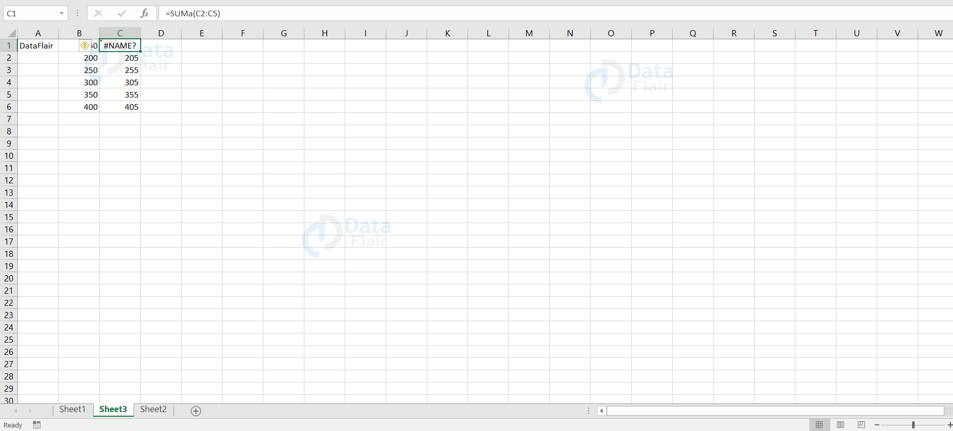
How to Correct #NAME Error
- Enter the formula correctly.
- Ensure that the quotation marks are balanced properly from left and right.
- Make sure that the colon is specified between the ranges.
To solve the error, click on the warning symbol provided at the side of the cell.
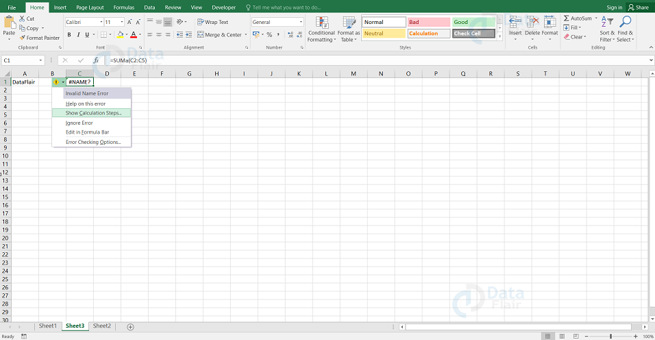
The list of options will appear and choose an option to resolve the error accordingly.
Ways to insert a formula in Excel
a. Simple Insertion in Excel
This is one of the most straightforward methods. In this insertion, the user should start typing the formula from typing an equal to sign. While typing the formula in excel, the preference appears and you can choose them if you want to and can finish the formula.
b. Quick Insert in Excel
Quick insert is one of the best options to use when you are performing the same type of calculation.
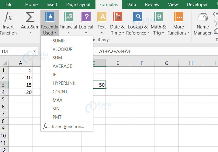
The recently used option contains the most frequently used formulas. To access the recently used option, click on the Formulas tab and choose the recently used option.
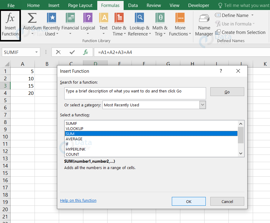
c. Insert Function from formulas tab
The user can insert formulas to a cell by using the insert function. To use the insert function, click on the Formulas tab, choose the insert function and select a function.
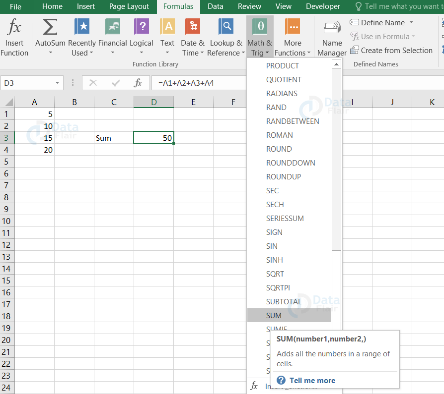
d. Selecting a formula from the group
The other way to perform calculations is to choose the formula from the groups provided in the MS-Excel. To choose a formula function from one among the options, then go to the Formulas tab, click on to the preferred group tab and choose the appropriate function.
The groups in MS-Excel are:
- Financial
- Logical
- Text
- Date & Time
- Lookup & Reference
- Math & Trig
Each group contains the formulae related to their group name.
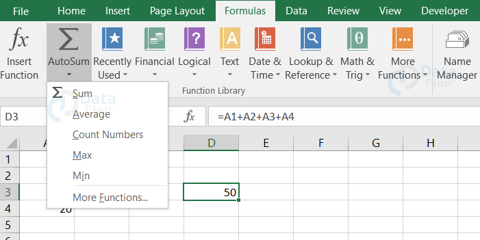
e. Autosum Option in Excel
You can use this option when you want to autocomplete your function. It’s just a one click away. To use the autosum option, click on the formulas tab, choose the autosum option and click on the required function.
Absolute Referencing in Excel
Absolute referencing is referencing which helps in accessing a particular value in different cells.
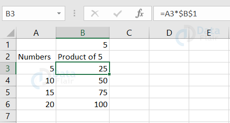
Here, we are multiplying the value in the cell with a particular value. The dollar symbol makes it an absolute reference.
Relative Referencing in Excel
Relative referencing is the referencing used when the cells should be shifted automatically for each calculation.
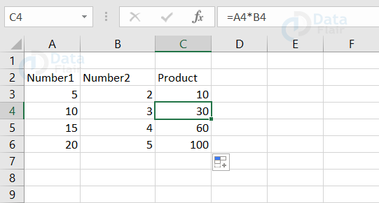
Here, we wanted to multiply the two numbers in A and B column cells. Using relative referencing, we need not type the formula every time. Instead, if you drag, the cells will be automatically filled with the assistance of relative referencing.
Mixed Cell References in Excel
If both the row and column references are relative and the other reference is absolute then, it is known as mixed cell references.
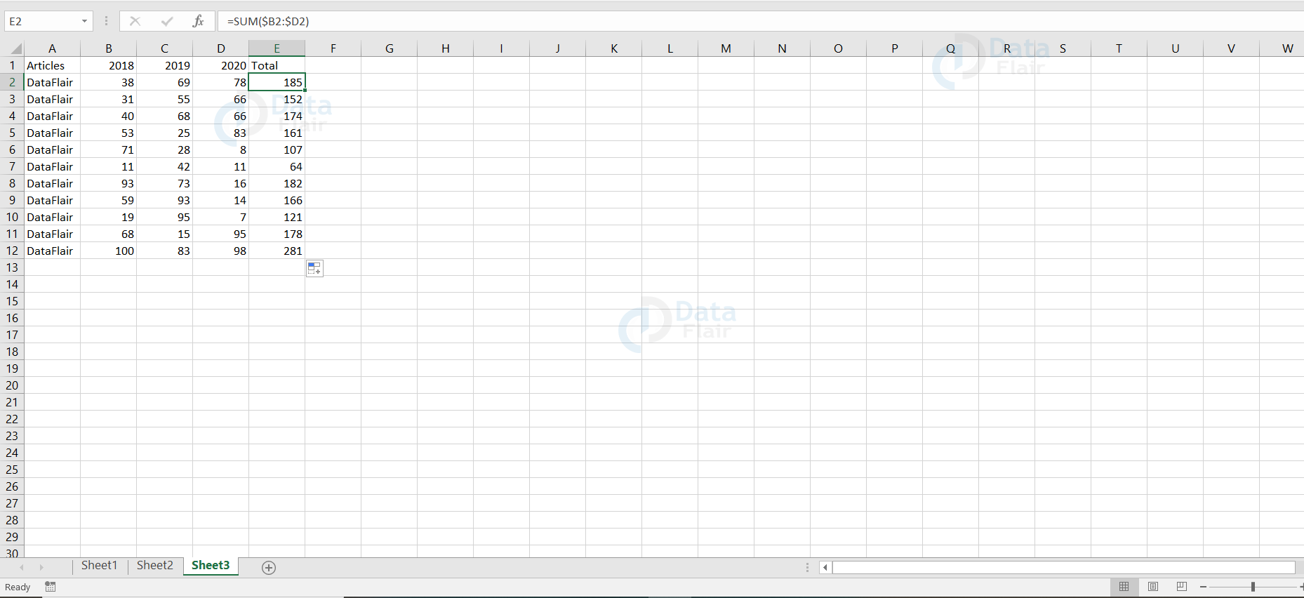
Here, the formula reference is made in such a way that it is relative to rows i.e., 2 and absolute to the columns i.e., B to D.
Some Basic Arithmetic Excel Formulas
Using the data values in the workbook, we will see how arithmetic operators perform its calculation.
Here A1 = 20, A2 = 10
| Operation | Operator | Example | Description |
| Addition | + | =A1+A2 Output =30 | Summing of two values in the cells A1 and A2. |
| Subtraction | – | =A1-A2 Output =10 | Subtraction of the value in the cell A2 from A1. |
| Multiplication | * | =A1*A2 Output =200 | Product of two values in the cells A1 and A2. |
| Division | / | =A1/A2 Output =2 | Dividing the value of cell A1 by the value in cell A2. |
| Percentage | % | =A1*A2% Output =2 | To find A2% of the number in the cell A1. |
| Exponentiation | ^ | =A1^A2 Output =1.024E+13 | Raising of the value in A1 by the power of A2. |
| Negation | – | =-A1 Output =-20 | A1 value will be represented with a minus symbol before it. For example if A1 contains the value 5, then the negation value is -5. |
What is Function in Excel?
Functions are the formulas that are predefined and these are used for specific values in a particular order. It is very useful to perform quick tasks such as calculating the sum, average, count, minimum, maximum values, etc.
Importance of functions in Excel
1. Function makes the calculations easier and it increases user productivity.
2. If the user calculates the sum of a few cells, then the user has to reference all the cells one by one in the formulas whereas with a function, the start cell and end cell is all enough to calculate the sum. It makes it a lot easier rather than referencing a lot of cells.
Text functions in Excel
Some of the text functions in MS excel are:
| Function | Formula | Example | Description |
| LEFT | =LEFT(Text, Number_of_Characters) | =left(“DataFlair”,6) Output =DataFl | This function returns the specified number of characters beginning from the left side of the string. |
| RIGHT | =RIGHT(Text, Number_of_Characters) | =right(“DataFlair”,5) Output =Flair | This function returns the specified number of characters beginning from the right side of the string. |
| MID | =MID( Text, Start_number, Number_of_Characters) | =mid(“DataFlair”,1,4) Output =Data | This function returns the specified number of characters beginning from the mid of the string. |
| ISTEXT | =ISTEXT(Cell) | =istext(“DataFlair”) Output =True | This function returns true if the cell contains text value or else it returns false. |
| FIND | = FIND(Text, within_Text, [Start_position]) | =FIND(“Fl”,”DataFlair”,1) Output =5 | This function returns the starting position of the specified search in the other string. The 1 in the function specifies the index number from where the function starts. |
| REPLACE | =Replace(“old_string”, start_position, number_of_characters, “new_string”) | =REPLACE(“Sun”,1,1,”B”)Output =Bun | This function replaces a part of a string. |
| SUBSTITUTE | =Substitute(old_string, new_string, [index_position]) | =SUBSTITUTE(H17,”Sun”,”Bun”)Output =Bun This output appears if the H17 cell contains the word “sun”. | This function substitutes a part of a string. |
Numeric Functions in Excel
Some of the numeric functions in Excel are
| Function | Formula | Example | Description |
| ISNUMBER | =ISNUMBER(Value) | =ISNUMBER(25) Output: True | This function checks whether the value is a numeric data type or not. If it is numeric, it returns true or else it returns false. |
| ROUND | =Round(Number,num_digits) | =round(102.322343,2) Output: 102.32 | This function rounds a number to a specified number of digits. |
| RAND | =Rand() | =Rand() Output: 0.2 | This function returns a value between 0 and 1. |
| POWER | =Power(number, power) | =power(5,2) Output: 25 | This function returns the value raising the number to the provided power value. |
| RANDBETWEEN | =Randbetween(bottom,top) | =Randbetween(10,20) Output: 17 | This function returns a value between the bottom and top number. |
| MEDIAN | =median(num1,num2…) | =median(2,3,4,5,6,) Output 4 | This function returns the middle most value of the numbers. |
| PI | =pi() | =pi() Output: 3.141593 | This function returns the pi value used for calculation. |
| ROMAN | =roman(number,[form]) | =roman(17,1) Output: XVII | This function returns the number value in the specified roman form. |
Logical Function in Excel
Some of the logical functions in MS Excel are:
| Function | Formula | Example | Description |
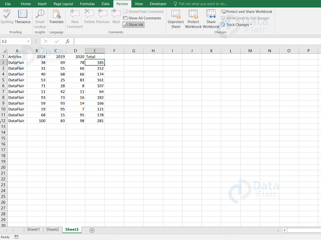
| AND | =AND(logical1,[logical2]…) | =AND(B2>80,C2>80,D2>80) Output: True | This function tests a number of conditions defined by the user and returns true only when all conditions are met or else it returns false. |
| OR | =OR(logical1,[logical2]…) | =OR(B2>80,C2>80,D2>80) Output: True | This function tests a number of conditions defined by the user and returns true if any one of the conditions is met or else it returns false. |
| NOT | =NOT(logical) | =Not(B2>80) Output: False | This function returns the opposite value of the logical expression which means the function returns false in the place of true and true in the place of false. |
| LARGE | =LARGE(Array,k) | =Large(B2:D2,3) Output:87 | This function returns the kth largest value. If k=1, it performs the same function as maximum. |
| SMALL | =SMALL(Array,k) | =Small(B2:D2,2) Output:90 | This function returns the k th smallest value. If k=1, it performs the same function as minimum. |
Date Time Functions in Excel
Some of the date-time functions in Excel are:
| Function | Formula | Example | Description |
| Date | =Date(year,month,day) | =Date(2021,5,21) Output =21-05-2021 | This function returns the numbers in the date format. |
| Days | =Days(end_date, start_date) | =DAYS(21-05-2021,21-03-2021) Output =61 | This function returns the number of days between those two dates. |
| Month | =month(cell) | =month(21-05-2021) Output =5 | This function returns the month number from the cell. |
| Minute | =minute(cell) | =minute(3:48) Output =48 | This function returns the minute from the cell value. |
| Second | =Second(Cell) | =Second(Now()) Output =41 This function tells you the second of now. | This function returns the second value from a time format data. |
| Hour | =Hour(cell) | =Hour(NOW()) Output =10 This function tells you the hour of now. | This function returns the hour number from 0 to 23. |
| Datedif | =datedif(start_date,end_date, “y/m/d”) | =datedif(31-12-1999,24-05-2021) Output =21 | This function provides you the difference between two dates. It denotes the differences in terms of years, months or days. |
| Time | =Time(Hour,Minute,Second) | =Time(12,22,32) Output =12:22PM | This function converts the hour,minute,value to the time format. |
| DateValue | =Datevalue(date_Text) | =Datevalue(4/10/1975) Output =27464 | This function converts the date to a serial number. |
| TimeValue | =Timevalue(date_Text) | =Timevalue(“9:00”) Output =0.375 | This function converts the time to a serial number. |
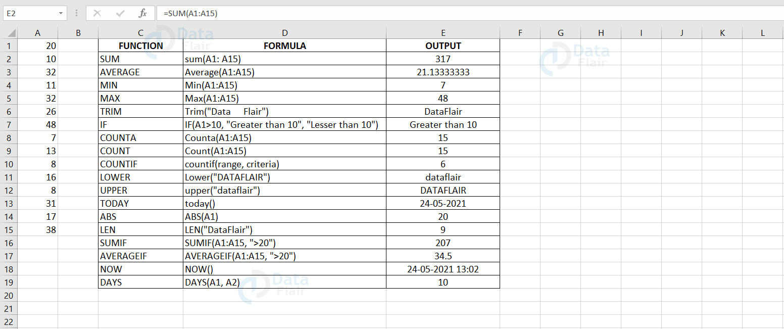
Basic Formulas and Functions in Excel
Excel formulas help the user to decrease the amount of time they spend in Excel and increase the accuracy of the data and reports.
| Formula Name | Formulas | Example | Description |
| Sum | =sum(Start cell: End cell) | =sum(A1: A15) Output =317 | It sums up the value of the cells from the start to the end cell. |
| Average | =Average(Start cell: End cell) | =Average(A1:A15) Output =21.31333 | This function finds the average of the specified cells. |
| Min | =Min(Start cell: End cell) | =Min(A1:A15) Output =7 | It fetches the minimum value from the ranged cells. |
| Max | =Max(Start cell: End cell) | =Max(A1:A15) Output =48 | It fetches the maximum value from the ranged cells. |
| Trim | =Trim(Text) | =Trim(“Data Flair”) Output =DataFlair | This function helps you to eliminate the spaces. It works on only one cell at a time. |
| If | =IF(logical_test, [value_if_true],[value_if_false]) | =IF(A1>10, “Greater Than 10” , “Lesser Than 10”) Output =Greater Than 10 | This helps you to sort your data according to the logic. |
| Counta | =Counta(Start cell: End cell) | =Counta(A1:A15) Output =15 | This function counts the number of cells that are not empty in the specified range. |
| Count | =Count(Start cell: End cell) | =Count(A1:A15) Output =15 | This function counts all the numeric values in the specified range. |
| Countif | =countif(range, criteria) | =countif(A1:A15, “>20”) Output =6 | This function counts the values if it meets the criteria in the specified range |
| Proper | =Proper(Text) | =PROPER(“dataflair”) Output =Dataflair | This function converts the text into a proper case which is starting the word with a capital letter and being continued by small letters. |
| Lower | =Lower(Text) | =Lower(“DataFlair”) Output =dataflair | This function converts the text into lowercase. |
| Upper | =upper(Text) | =Upper(“DataFlair”) Output =DATAFLAIR | This function converts the text into uppercase. |
| Today | =today() | =Today() Output =24-05-2021 | This function returns the current date in the cell. |
| ABS | =ABS(cell number) | =abs(A1) Output =20 | ABS function returns the absolute value of the cell without affecting its data type. |
| LEN | =LEN(cell number) | =LEN(“DataFlair”) Output =9 | This function returns the count of number of characters in a string text |
| SUMIF | =SUMIF (range, criteria, [sum_range]) | Sumif(A1:A15, “>20”)
Output =207 | This function adds all the values which meet the specific criteria in a range of cells. |
| AVERAGEIF | =AVERAGEIF(range, criteria, [average_range]) | Averageif(A1:A15, “>20”) Output =34.5 | This function calculates the average value which meets the specified criteria in a range of cells. |
| NOW | =NOW() | =NOW() Output =24-05-2021 13:02 | This function returns the current date and time of the system |
| DAYS | =DAYS(end_date, start_date) | =DAYS(A1, A2) Output =10 | This function returns the count of the number of days between two dates |
Math & Trig Functions in Excel
Some of the Math and Trig Functions are:
| Function | Formula | Example | Description |
| ABS | =Abs(number) | =abs(-1) Output: 1 | It returns the absolute value of the specified number. |
| SIGN | =Sign(number) | =sign(-10) Output: -1 | It returns the sign of a specified number through -1,0,+1. If it is negative, it returns -1, 0 if the number is zero and 1 if the number is positive. |
| SQRT | =Sqrt(number) | =Sqrt(5) Output: 2.23 | It returns the square root of a number |
| MOD | =mod(number,divisor) | =mod(10,3) Output: 1 | It returns the remainder after the division. |
Excel Creating Formulas
The user can create formulas as per their convenience in the spreadsheets.
Let’s look at a sample,
The B1 cell holds the value 150. Now, let’s type the formula =B1 + 100 in the C1 cell and press the enter key.
The following output appears.
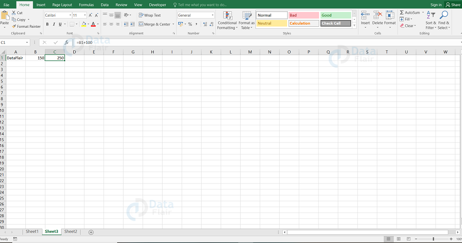
The formulas in the cell add 100 to the B1 cell value and the result appears in the C1 cell.
In a similar way other formulas can be created:
=B1 * 100 for multiplication, the value in the cell B1 is multiplied with 100.
=B1 – 100 for subtraction, 100 is subtracted from the value in the cell B1.
More formulas can be created by typing = in the desired cell and refer to the appropriate cell in the formulas cell.
See the formula created to calculate the difference between the cells.
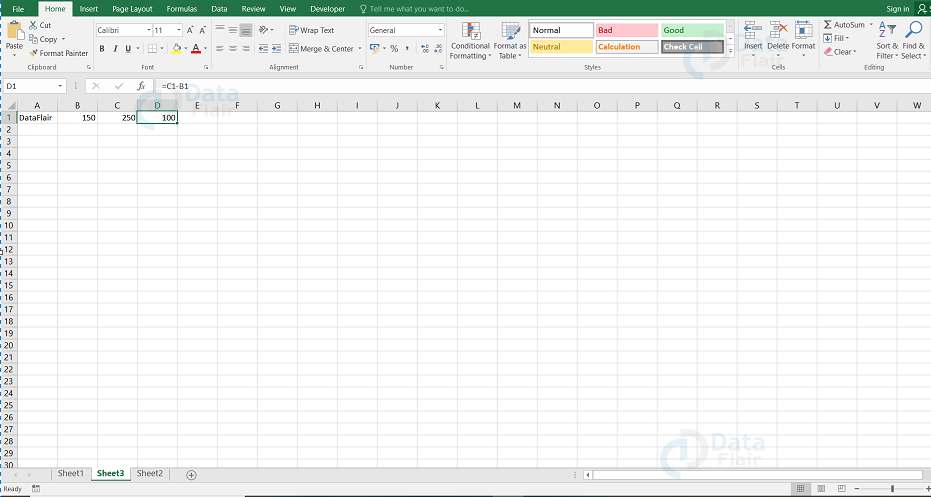
Edit a Formula in Excel
You can also edit a formula of the cell in the formula bar. When you click on the cell, the formula of that particular cell appears in the formula bar.
Click on the formula and make the required changes.

Once the changes are made, press enter.
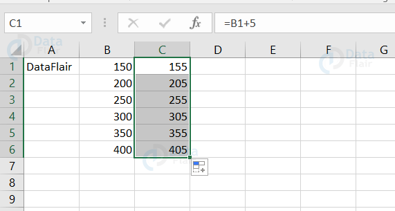
Excel Fill Handle in Formulas
The user can write the formula in one or few cells. But writing the same formula more times is going to be time consuming and hence to overcome this, the excel has a feature which helps the user to fill the cells.
The user uses the fill handle to perform the calculations. So, type the formula =B1+5 in cell C1 then drag the cursor by placing it on the right bottom corner of cell C1, fill handle will appear. Drag it till where it is required and here it is until C6. The whole list of numbers in column B will be added by 5.
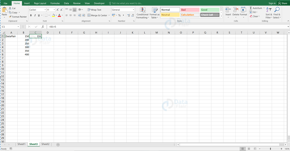
Once you drag the cursor, the following output appears.
1. Copy and paste formulas
If you want to copy paste formulas, right click on the cell and choose the copy option. After that, go to your desired cell, right click on it and choose the paste option. When we copy paste the formula, it automatically adjusts the cell references.
2. Hide Formulas in Excel
In case you want to hide some formula from an excel sheet, you can do it using below steps:
1: Right click on the cell which you want to hide.
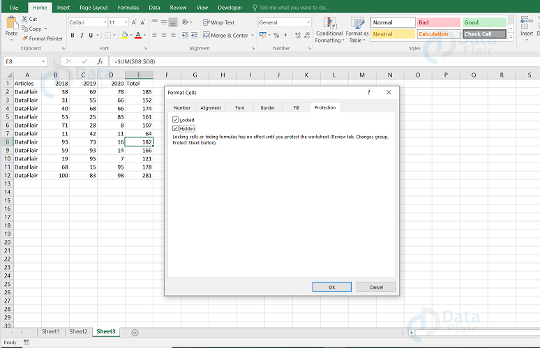
2: Click on the format cells and go to the protection pane.
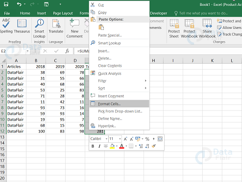
3: Tick on the checkbox beside the hidden option and press ok.
4: Go to the review tab and click on the protect sheet.
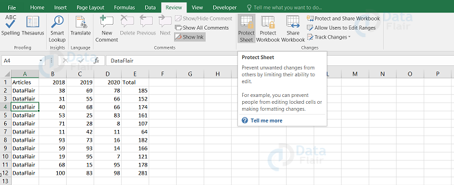
5: It will ask for a password and once this is done, the formula will be in protected mode.
The formula is not visible now in the formula bar.
Note: To unhide the formula, you have to unhide the worksheet with the password.
3. Combining Functions
You can use more than one function in a cell itself. Using more than one function in a cell is said to be nested functions.
Let’s look at a sample:
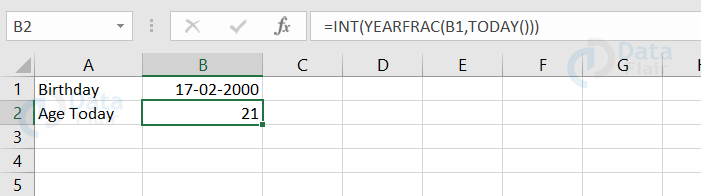
Here, we are trying to find the age using functions such as int,yearfrac,today. Notice that the today function is inside the yearfrac and this is called nesting. We are using int here to obtain the value in a whole number.
Instruction while typing data in excel
To make the formulas work, enter the values and text in separate cells.
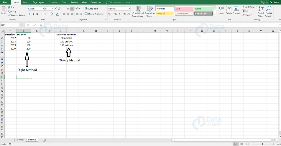
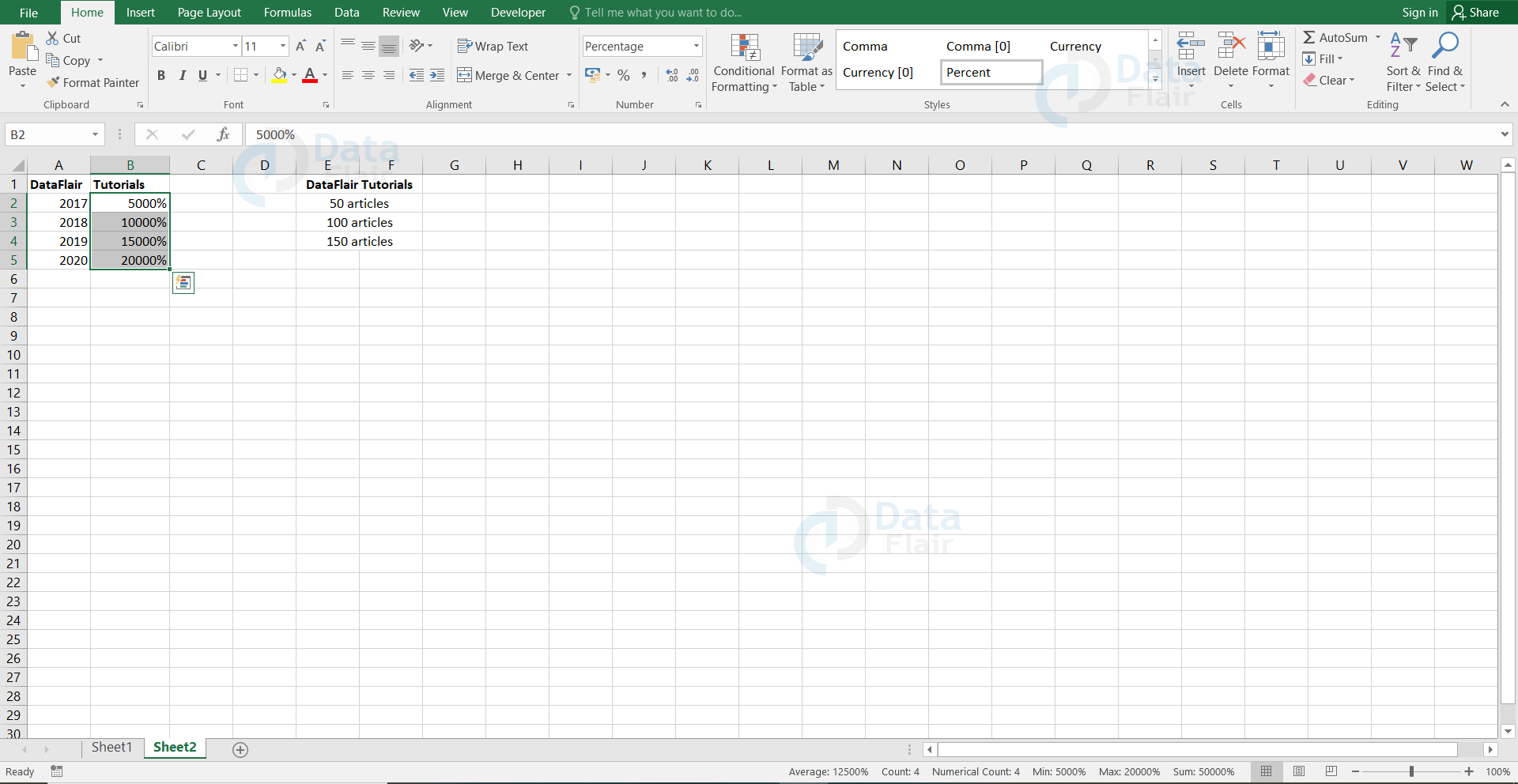
In case you want to add percentage symbols to the B column values then use the mini toolbar.
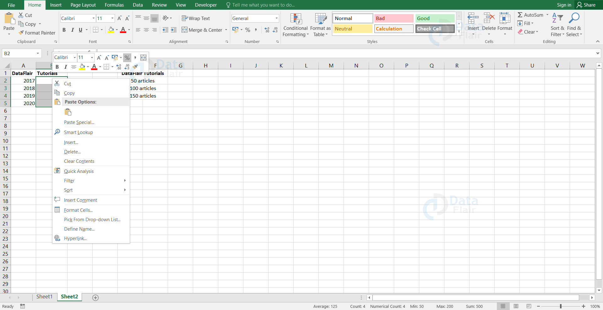
Right click on the range of cells, the mini toolbar appears above the shortcut menu. Click on the percentage symbol and that will be added to the given range.
Quick Excel Functions
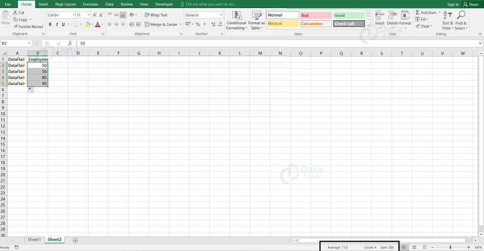
There are some quick functions in Excel such as status bar quick functions which provide the user with the statistics of the worksheet without using formulas.
When the user selects the desired range, the statistics appear in the status bar. The information such as the average, the count, and the sum of the cells are available.
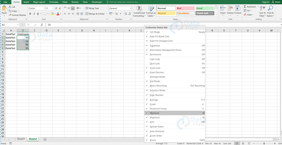
Note: The user can customize the status bar by right-clicking on it. The user can add more functions in the status bar. In order to do that, select the function from the menu list which you want to add in the status bar and then even those functions will appear in the status bar.
Advanced Functions in Excel
Advanced Functions in MS Excel are:
| Function | Formula | Example | Description |
| PV | =PV(rate,nper,pmt,[fv],[type]) | =PV(0.02,20000,10) Output =-500.00 | This function helps you to calculate the rate, investment period payments, future value and others based on the input you provide. |
| CONVERT | =Convert(number, from_unit, to_unit) | =CONVERT(9000,”g”,”kg”) Output =9 | This function converts from one unit to the other unit. Here, we are converting it from grams to kilograms. |
| TYPE | =TYPE(Cell) | =TYPE(90) Output =1 | This function returns the type of the data in the cell. Here, it returns 1 as it is an integer. |
| REPT | =REPT(Text, Number_Times) | =REPT(“DataFlair”,2) Output =DataFlairDataFlair | This function helps in repeating the same value in the cell. Here, the text “DataFlair” is repeated twice. |
| CHOOSE | =CHOOSE(index_number, value1,value2..) | =CHOOSE(1, A, B, C) Output =A | This function comes to action when there are two outcomes for a particular condition. |
| CONCATENATE | =CONCATENATE( Text1, Text2) | =CONCATENATE(Data, Flair) Output =DataFlair | This function is used to combine two or more cell values together in a new cell. |
CEILING | =CEILING(number, multiple_significance) | =CEILING(23.45,5) Output =25 | This function returns the round off value nearer to the significance multiple. Here, 5 is the multiple significance. |
FLOOR | =FLOOR(number, multiple_significance) | =FLOOR(23.45,5) Output =20 | This function returns the value, rounding down to the nearest significance. |
Some of the other Excel Advanced Functions are:
| Function | Formula | Example | Description |
SUBTOTAL
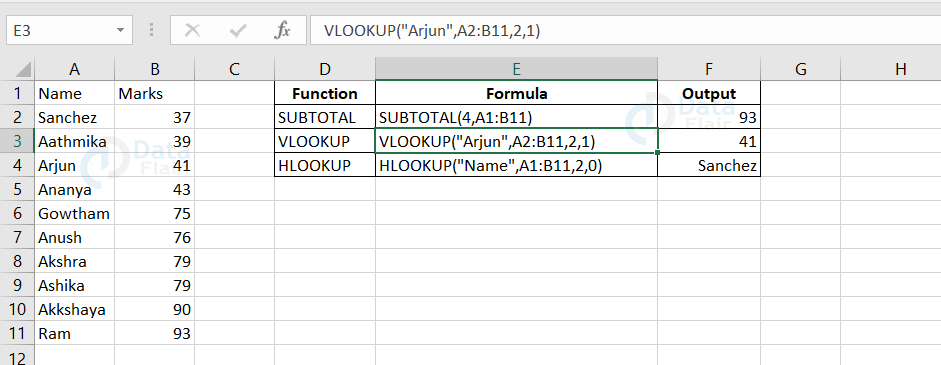
| =SUBTOTAL(FUNCTION_REFERENCE, VALUE1,VALUE2..) | =SUBTOTAL(4, A1:B11) Output =93 | This function helps you to perform various activities for a database.You can perform any of the functions such as average,max,min, etc using subtotal function. Here, the 4 is the reference to maximum function. |
| VLOOKUP | =vlookup(lookup value, table array, column index number, range lookup) | =vlookup(“Arjun”,A2:B11,2,1) Output =41 | This function returns the value from the column you specify. |
HLOOKUP | =hlookup(lookup value, table array, row index number, range lookup) | =hlookup(“Name”,A1:B11,2,0) Output =Sanchez | This function returns the value from the row you specify. |
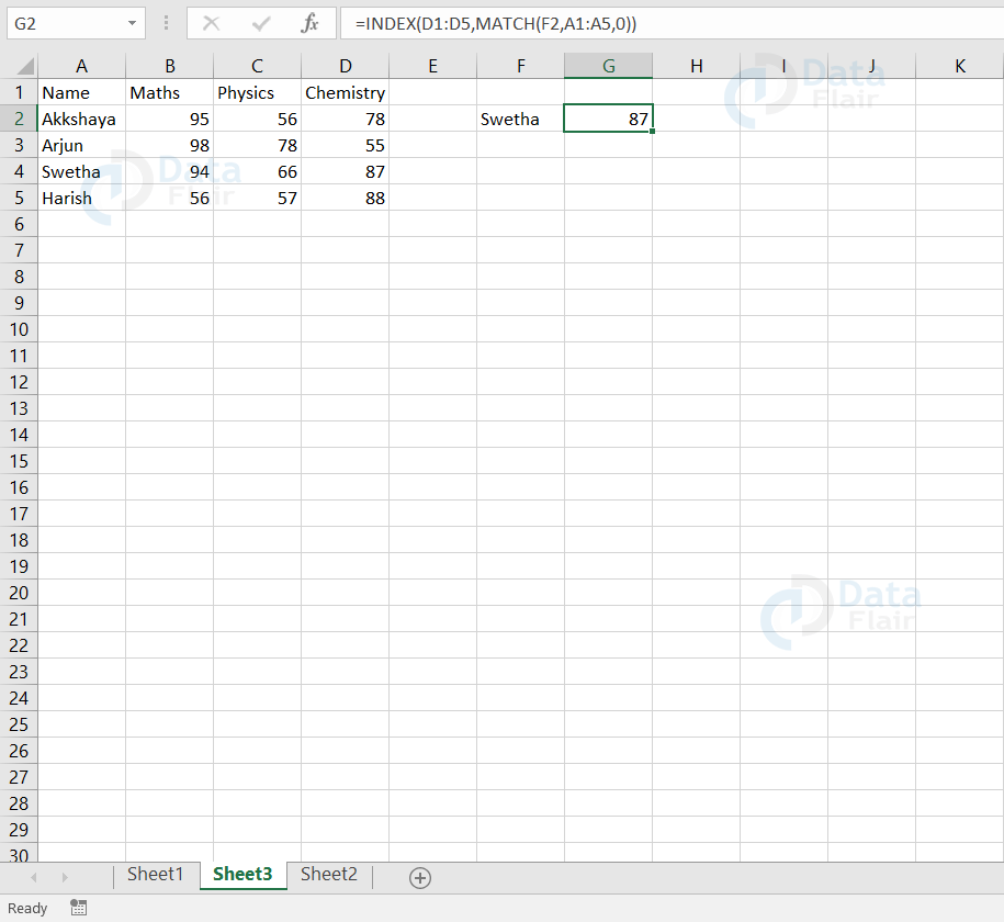
Index Match in Excel
Index-Match function helps the user to find value in a column to the left. The user also uses index-match often because it requires less processing power compared to the vlookup function. In vlookup function, it has to evaluate the entire table array and whereas in index match, excel has to consider the lookup column and return value only.
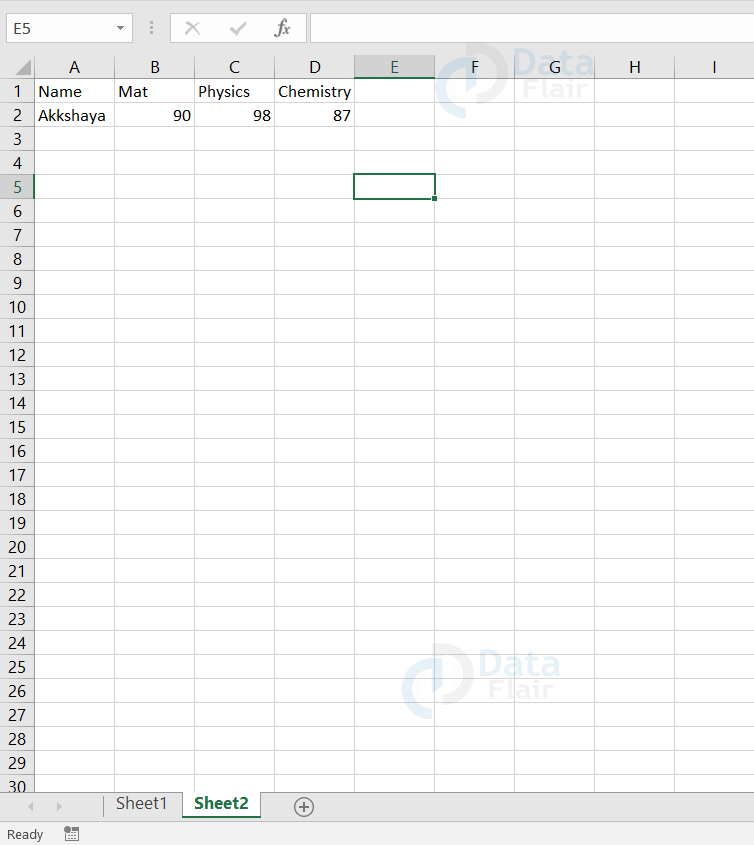
From the following table, let’s find the chemistry marks of swetha.
=INDEX(D1:D5,MATCH(F2,A1:A5,0))
Summary
1. Using formulas and functions, we can analyze the data.
2. The data can be formatted and it can be maintained for the long term.
3. Functions provide you more accurate values because the mistakes that may happen in function are quite lesser than the formula.
4. Formula bar helps you in viewing the calculation in a particular cell.
Did you like our efforts? If Yes, please give DataFlair 5 Stars on Google


