Divide and Conquer Algorithm

Have you ever been a part of the annual fest organizing committee at your college or your institution? If not, allow me to tell you how to organize a large-scale annual fest efficiently at any institution.

There are mainly two tasks while organizing a fest. Decorating the campus and organizing events. Now the event organizer cannot do these huge tasks alone, so the organizer assigns these two tasks to two different people.

Event coordinator-1 volunteers for the task of decorating the whole campus and another person, event coordinator-2 gets the task of organizing all the events. Now further these two persons cannot complete the task. So they divide their task into sub-members of the committee.

A group of people gets to make banners for decoration and another group gets to put all the lights all over the campus. The third group gets to organize the gaming events and the last group gets the task to organize the talk shows events.

Now they achieve their task separately, combine them and at the end, we have a very well organized annual fest which you are going to remember for years to come. This is a very good example of divide and conquer.

When a single task is very huge to execute, the problem is divided into multiple subproblems. Each problem is then solved individually and at the end combined to get the solution to the whole problem.

In this article, we will study the divide and conquer algorithm, its fundamentals, and its pros and cons. We shall also see some very good real-life applications of the divide and conquer algorithm approach.

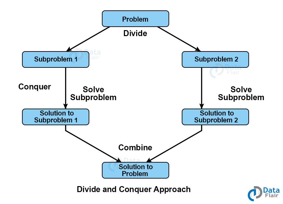
Divide and Conquer Algorithm

In the divide and conquer algorithm, the problem is divided into multiple subproblems. Each subproblem is then solved, and then combine all the solutions to these subproblems to get the solution of the whole problem. 

This algorithm has three steps:

1. Divide: divide the larger problem into multiple subproblems.

2. Conquer: recursively solve every subproblem individually.

3. Combine: combine all the solutions of all the subproblems to get the solution to the whole problem.

Fundamentals of divide and conquer algorithm

The divide and conquer strategy of designing algorithms has two fundamentals :

• Relational formula
• Stopping condition 

1. Relational formula

It is the formula generated from a given technique. After generating the formula, we apply the divide and conquer strategy to break the problem into many subproblems and solve them individually.

2. Stopping condition

When you divide the problem by divide and conquer strategy, you need to understand for how long you have to keep dividing. You have to put a stopping condition to stop your recursion steps.

Divide and conquer recurrence relations

Recurrence relation for divide and conquer is given by:

T(n) = aT(n/b) + f(n), where a > 1 and b > 1

We solve the above recurrence relation using the Master Method. It is a direct way of getting a solution to recurrence relations for divide and conquer algorithms. There are three cases:

1. If f(n) = Θ(n^c) where c < log_ba then T(n) = Θ(n^logba)
2. If f(n) = Θ(n^c) where c = log_ba then T(n) = Θ(n^clog n)
3. If f(n) = Θ(n^c) where c > log_ba then T(n) = Θ(f(n))

Let a recurrence relation be  : 

T(n) = 2T(n/2) + cn. Here a=2,b=2,k=1.

Log_ba = log₂2 =1 = k.

Complexity :  Θ(nlog2(n))

For example:

For merge sort: recurrence relation : T(n) = 2T(n/2) + Θ(n). Here, c=1 and log_ba=1.  The complexity of merge sort come out to be Θ(n log n).

Advantages of Divide and Conquer Algorithm

1. Divide and conquer successfully solved one of the biggest problems of the mathematical puzzle world,  the tower of Hanoi.

You might have a very basic idea of how the problem is going to be solved but dividing the problem makes it easy since the problem and resources are divided.

2. Is very much faster than other algorithms.

3. The divide and conquer algorithm works on parallelism. Parallel processing in operating systems handles them very efficiently.

4. The divide and conquer strategy used cache memory without occupying much main memory. Executing problem in cache memory which is faster than main memory.

5. Brute force technique and divide and conquer techniques are similar but divide and conquer is more proficient

Disadvantages of Divide and Conquer Algorithm

1. Most of the divide and conquer design uses the concept of recursion therefore it requires high memory management.

2. Memory overuse is possible by an explicit stack.

3. It may crash the system if recursion is not performed properly.

Divide and conquer algorithm vs dynamic programming

Both divide and conquer and dynamic programming divides the given problem into subproblems and solves those problems. Dynamic programming is used where the same problem is required to be solved again and again, whereas divide and conquer is used where the same problem is not required to be calculated again.

For example, in the merge sort algorithm, we don’t need to calculate the same subproblem again, but while calculating the Fibonacci series we need to calculate the sum of the past two numbers again and again to get the next number. So we use dynamic programming in this case.

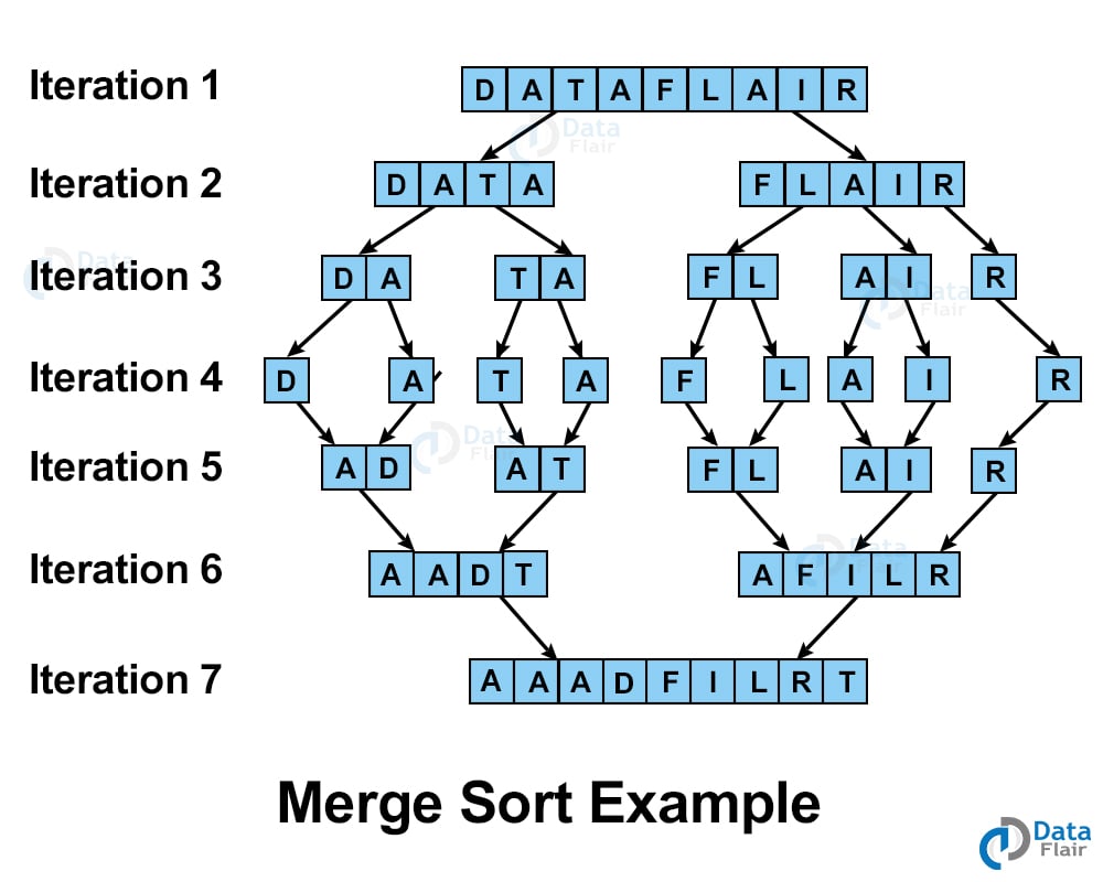
Let us see an example for better understanding.

Arrange the letter of the word “DATAFLAIR” alphabetically using the merge sort technique.

Writing a function in Dynamic programming to generate Fibonacci series:

member=[ ]
fibonacci(n)
           If  n in member: return member[n]
          else,     
                  If n < 2, f = 1
                   else , f = f(n - 1) + f(n -2)
                    mem[n] = f
                    return f

Writing a function using divide and conquer approach to generate Fibonacci series:

fibonacci(n)
    If n < 2, return 1
    Else , return f(n - 1) + f(n -2)

Max-Min problem Analysis

Traditional algorithm for finding max, min element in an array:

findmaxmin (a [ ])
Max = a [0]
Min =  a [0]
For i= 1 to n-1 do
    If a[i] > max then
          max = a[i]
    if a[i] < min then
          Min = a[i]
return (max, min)

In the above method, the number of comparisons between elements is 2n-2.

In a divide and conquer approach for finding maximum and minimum elements, we divide the problem into subproblems and find max / minor for each subproblem. And in the next step, the outputs of individual subproblems are compared again to get results.

Let n = size of the array

Let T (n) = time required to execute an algorithm on an array of size n. Divide terms as T(n/2)

‘2’ here tends to the comparison of the maximum with maximum and minimum with minimum as in the above example.

T(n) = T(n/2 ) + T(n/2) + 2                                  …(1)

T (2) = 1, time taken to compare two elements.

T(n/2) = 2T(n/2²) + 2                                            …(2)

Put (2) in (1):

T(n) = 2 [ 2T (n/2²) + 2 ] + 2

       = 2² T( n/2²) +2² + 2

Applying  the same procedure recursively on each subproblem we get:

T(n) = 2ⁱ T( n/2ⁱ ) + 2ⁱ + 2^i-1 + ……………. + 2          …(3)

Terminate at:  ( n/2ⁱ ) = 2 n = 2ⁱ⁺¹               … (4)

Put (4) into (3).

T(n) = 2ⁱT(2) + 2ⁱ + 2^i-1 + ……………. + 2

       = 2ⁱ.1 + 2ⁱ + 2^i-1 + ……………. + 2

       = 2ⁱ + (2(2ⁱ – 1)) / (2-1)

       = 2ⁱ⁺¹ +2ⁱ – 2

       = n + n/2 – 2

       = 3n/2 – 2

The number of comparisons required after the divide and conquering approach on n elements/items = ( 3n/2 – 2 ). This is less than the no. of comparisons in a traditional approach.

For example, array size=11

Traditional approach: (2n-2) = 20 comparisons

Divide and conquer approach: ( 3n/2 – 2 )= 14.5 ≈ 15 comparisons.

Applications of Divide and Conquer

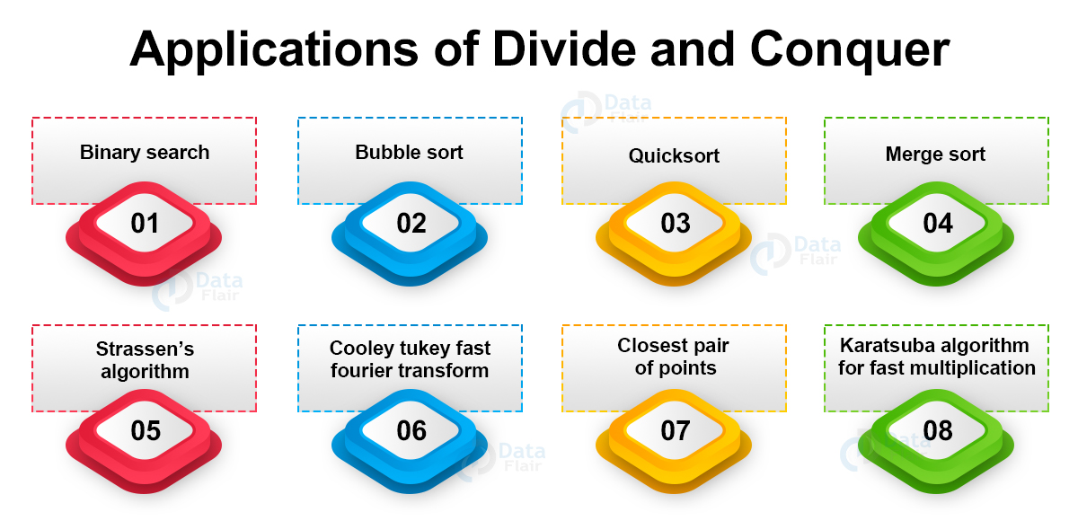
1. Binary search: Binary search is the fastest search algorithm requiring the only condition that the elements in the array are already arranged either in ascending or descending order.

Also known as half interval search, it compares the search element to the middle element. If the search element is less than the middle element, it selects the first half otherwise the second half.

The same process is recursively applied on the selected half of the array until the search element is found.

2. Bubble sort: Compare each pair of elements, and if they are not in order, then swap them. This sorting technique has a worst-case time complexity of O(n2) and therefore it is not suitable for large data sets.

While sorting, the last element is the first one to settle at its final position, and hence the modified algorithm does not include the last iteration in the loop after each iteration.

3. Quicksort: This most efficient sorting algorithm selects a pivot value from an array and divides the rest of the array elements into two subarrays. It compares the pivot element to each element and sorts the array recursively.

4. Merge sort: This algorithm divides the array into sub-arrays and then recursively sorts them. After sorting it merges them back.

5. Strassen’s algorithm: Named after Volker Strassen, this is an algorithm for matrix multiplication that is much faster than a traditional algorithm used for large matrices. 

This method implies 7 recursive calls. It divides the matrices of order N into sub-matrices of order N/2 and calculates the sub-matrices of resultant matrices according to the following equations: 

p1 = a(f-h)                       p2 = (a + b)h                        

p3 = (c + d)e                   p4 = d(g- e)

p5 = (a + d)(e+ h)          p6 = (b-d)(g+h)

p7 = (a-c)(e+f)

6. Cooley Tukey Fast Fourier Transform: Named after J.W. Cooley and John Turkey. It is the most common FFT algorithm based on the divide and conquer approach. It works in O(n log n)  time complexity.

7. Closest pair of points: This is a problem of computational geometry focusing on finding out the closest pair of points in metric space, given n point, such that the distance between the pair of points is minimum.

8. Karatsuba algorithm for fast multiplication: Invented by Anatoly Karatsuba in late 1960, this is one of the fastest multiplication algorithms of the traditional time. It performs multiplication of two n digit numbers in at most a single-digit multiplication in general. 

We divide the numbers into two halves. Let numbers be X and Y:

   X =  Xl*2n/2 + Xr    

Y =  Yl*2n/2 + Yr

Here,

 Xl, Yl: contains leftmost N/2 bits of numbers X and Y respectively.

Xr, Yr : contains rightmost  N/2 bits of numbers X and Y respectively

XY = 2n XlYl + 2n/2 * [(Xl + Xr)(Yl + Yr) – XlYl – XrYr] + XrYr

The complexity of the above equation is O(n^1.59) which is better than the time complexity of the traditional approach (O(n^2)).

Conclusion

In this article, we observed some real-life applications of the divide and conquer approach for designing algorithms. We also solved an example for merge sort. After this article, we are now aware of the differences between the divide and conquer approach and the dynamic programming approach.

Solving recurrence relations to calculate the time complexity is also covered here. We also learned about the types, and advantages, and disadvantages of divide and conquer.