Distance Vector Routing vs Link State Routing
Interactive Online Courses: Elevate Skills & Succeed Enroll Now!
Routing is the process of transferring data from a source to a destination over the internet. The two types of routing algorithms are distance vector routing and link state routing, which are classified based on how the routing tables are updated.
The first distinction between distance vector and link state routing is that in distance vector routing, routers share the knowledge of the entire autonomous system, whereas in link state routing, routers only share the knowledge of their immediate neighbours.
1. Distance Vector Routing:
Distance Vector Routing protocols determine the best path to a given destination based on distance. The distance metric is usually measured in hops, but it could also be delay, packet loss, or something else. If the distance metric is hop, a hop is traversed each time a packet passes through a router. The route to a given network with the fewest hops is the best route to that network.
The direction of that specific network is shown by the vector. Directly connected neighbours receive the entire routing table sent by distance vector protocols. RIP (Routing Information Protocol) and IGRP (Internal Gateway Routing Protocol) are two examples of distance vector protocols.
It’s a dynamic routing algorithm in which each router calculates the distance between itself and each potential destination, or its immediate neighbours.
The router shares its knowledge of the entire network with its neighbours, and the table is updated accordingly.
Information sharing takes place with neighbours on a regular basis.
Bellman-Ford algorithm helps in creating routing tables.
Operation:
All of the routers are turned on at the same time and run the same distance vector routing protocol. Each router communicates with its neighbour by sending its distance vector. Each router also receives distance vectors from each of its neighbours. The best estimate route to a given destination is inserted into the routing table by combining the information learned from neighbours with each router’s own information.
Example: We have a Router H, with neighbours A, B, F, G, I.
Now, let us assume:
a. Router H was informed by Router A and Router G that Router D is only 1 hop away.
b. Router H recognises that both routers (A and G) are neighbours, so it multiplies the hop metric by one.
c. Thus, Router H concludes that it can reach Router D via Router A and Router G in two hops.
Problems in Distance Vector Routing:
- A problem of counting to infinity is solved by splitting the horizon.
- Persistent looping problem, i.e. the loop will continue to exist indefinitely.
Characteristics of RIP (A Distance Vector Protocol):
- To maintain network integrity, RIP broadcasts every 30 seconds.
- RIP keeps routing tables, which show how many hops there are between routers, and is limited to 15 hops.
- When a router uses RIP, it sends its entire routing table to every directly connected neighbours router it recognises.
Key Properties of Distance Vector Routing:
a. Knowledge of the entire network:
Each router shares its information with the rest of the network. The Router shares the information it has gathered about the network with its neighbours.
b. Only sending network information to neighbours:
The router only sends network information to routers with direct links to it. Through the ports, the router sends whatever information it has about the network. The router receives the data and uses it to update its own routing table.
c. Sharing information on a regular basis:
The router sends the information to the neighbouring routers in 30 seconds.
Routing Table:
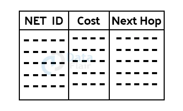
a. NET ID:
The Network ID identifies the packet’s final destination.
b. Cost:
The number of hops a packet must travel to reach its destination determines the cost.
c. Next Hop:
It is to this router that the packet must be sent.
Updating the Routing Table:
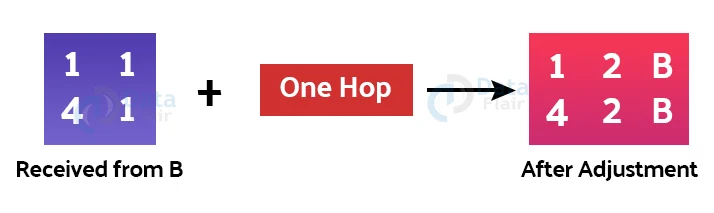
Suppose Router A sends its routing table to B, and a packet has to be sent from network 1 to 4. Then the update happens as follows:
- When A receives a routing table from B, it updates the table with the information it has.
- B’s routing table depicts how packets can be routed to networks 1 and 4.
- Because the B router is a neighbour of the A router, packets from A to B can be delivered in a single hop. As a result, 1 is added to all of the costs listed in B’s table, and the total is the cost of reaching a specific network.
2. Link State Routing:
Shortest-path-first protocols are another name for Link State protocols. Protocols that use link state routing have a complete picture of the network topology. As a result, they have a better understanding of the entire network than any distance vector protocol.
Each router with link state routing creates three separate tables. One table stores information about directly connected neighbours, another stores the topology of the entire internetwork, and the third stores the actual routing table.
All routers in the network receive information about directly connected links via link state protocols. OSPF (Open Shortest Path First) and IS-IS (Intermediate System to Intermediate System) are two examples of Link State Routing Protocols.
It is a dynamic routing algorithm in which each router in the network shares information about its neighbours with all other routers. Through flooding, a router sends information about its neighbours to all other routers. Information sharing happens only when there is a change.
Dijkstra’s Algorithm helps in creating routing tables.
Operation:
Link State Routing executes the following steps in its operation:
a. Discovery:
Each Link State enabled router sends a HELLO message on each of its links on a regular basis. Neighbour routers identify themselves in response to these HELLO messages. The HELLO initiator uses the network addresses of the routers to build up its neighbour table, which are attached to the replies.
b. Link Cost:
Each router is subjected to a series of tests in order to determine the cost to each of its neighbours. End-to-end delay, throughput, or a combination of these metrics could be used to calculate the cost. The important thing to remember is that every link state enabled router must have a cost estimate for each of its links.
c. Link State Packets:
Each router creates a packet containing its neighbours as well as the link costs associated with these neighbours. Each router adds its identity, a sequence number, and an age parameter to the beginning of the packet, the latter being used to ensure that no packet wanders around for an indefinite period of time. The packet floods into the network after the construction process is completed.
d. Shortest Path:
A router can then use the Dijkstra algorithm to compute the shortest path to any given destination using all of the details from its link state table.
Problems of Link State Routing:
- Heavy traffic due to packet flooding.
- Flooding causes infinite looping, and the Time to Live (TTL) field solves this problem.
Characteristics of OSPF (A Link State protocol):
- Over time, it is a more cost-effective routing protocol than RIP because it involves less network traffic.
- Instead of sending entire tables to routers, it sends updates to individual tables.
- The IP section of the TCP/IP protocol suite, which is the most commonly used alternative to RIP, receives routing information.
Key Properties of Link State Routing:
a. Knowledge of the neighbourhood:
Rather than sending its routing table, a router only sends information about its immediate surroundings. To other routers, a router broadcasts its identity and the cost of directly attached links.
b. Flooding:
Every router on the internetwork sends information to every other router except its neighbours. Flooding is the term for this process. Each router that receives a packet copies it and sends it to all of its neighbours. Finally, a copy of the same information is sent to each router.
c. Information sharing:
A router only sends information to all other routers when the information changes.
Two Phases of Link State Routing:
a. Reliable Flooding:
Initial State: Each node is aware of the costs of its neighbours.
Final state: Each node has a complete understanding of the graph.
b. Route Calculation:
Dijkstra’s algorithm, also known as the Link state routing algorithm, finds the shortest path from one node to all other nodes in the network.
The Dijkstra’s algorithm is iterative, and it has the property that after k iterations, the least cost paths for k destination nodes are well known.
Difference Between Distance Vector Routing and Link State Routing:
| Distance Vector Routing | Link State Routing |
| No flooding, small packets and local sharing require less bandwidth. | More bandwidth required to facilitate flooding and sending large link state packets. |
| Uses Bellman-Ford algorithm. | Uses Dijkstra’s algorithm. |
| Less traffic. | More network traffic when compared to Distance Vector Routing. |
| Updates table based on information from neighbours, thus uses local knowledge. | It has knowledge about the entire network, thus it uses global knowledge. |
| Persistent looping problem exists. | Only transient loop problems. |
| Based on least hops. | Based on least cost. |
| Updation of full routing tables. | Updation of only link states. |
| Less CPU utilisation. | High CPU utilisation. |
| Uses broadcast for updates. | Uses multicast for updates. |
| Moderate convergence time. | Low convergence time. |
Summary
In this article, we looked at 2 prominent algorithms, the Distance Vector algorithm and the Link State algorithm. We looked at the key properties of each, and the methods of functioning of each.
Your opinion matters
Please write your valuable feedback about DataFlair on Google


