Data Validation in Excel
We offer you a brighter future with industry-ready online courses - Start Now!!
In this tutorial, let’s discuss what data validation is and how it can be implemented in MS-Excel. Let’s start!!!
What Is Data Validation in Excel?
Data Validation is one of the features in MS-Excel which helps in maintaining the consistency of the data in the spreadsheet. It controls the type of data that can enter in the data validated cells.
Data Validation in MS Excel
Now, let’s have a look at how data validation works and how to implement it in the worksheet:
To apply data validation for the cells, then follow the steps.
1: Choose to which all cells the validation of data should work.
2: Click on the DATA tab.
3: Go to the Data Validation option.
4: Choose the drop down option in it and click on the Data Validation.
Once you click on the data validation menu from the ribbon, a box appears with the list of data validation criteria, Input message and error message.
Let’s first understand, what is an input message and error message?
Once, the user clicks the cell, the input message appears in a small box near the cell.
If the user violates the condition of that particular cell, then the error message pops up in a box in the spreadsheet.
The advantage of both the messages is that the input and as well as the error message guide the user about how to fill the cells. Both the messages are customizable also.
Let us have a look at how to set it up and how it works with a sample.
Setting up the Input message in Excel
- Click on the input message tab in the box.
- Fill the title and message as per the requirement and convenience.
- Then, press OK button.
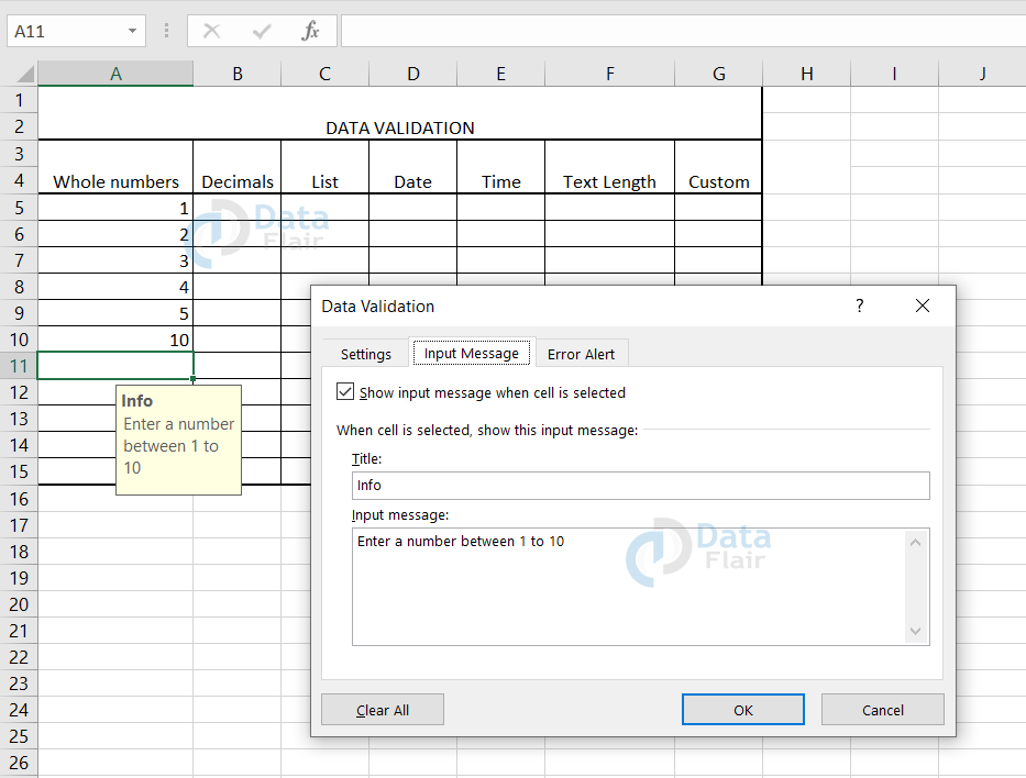
Here, the ‘info’ is the customised title and “Enter a number between 1 to 10” is the input message in this sample.
When you place the cursor on the data validation applied cell, the message will appear in a box as information.
Setting up the Error message in Excel
To set up the error message:
- Click on the error alert.
- Choose the style from the drop-down options.
We have three options here
- Stop
- Warning
- Information
This just changes the icon that appears in the box. It sets up the symbol as per the styling.
- Write the title and error message as you wanted it to appear.
- Then, click OK.
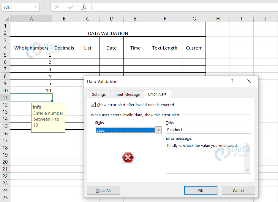
In this sample, “Re-check” is the title and “Kindly re-check the value you’ve entered” is the Error message here.
Once you press the ok button, the error alert message will pop up in a box when the user violates the data validation.
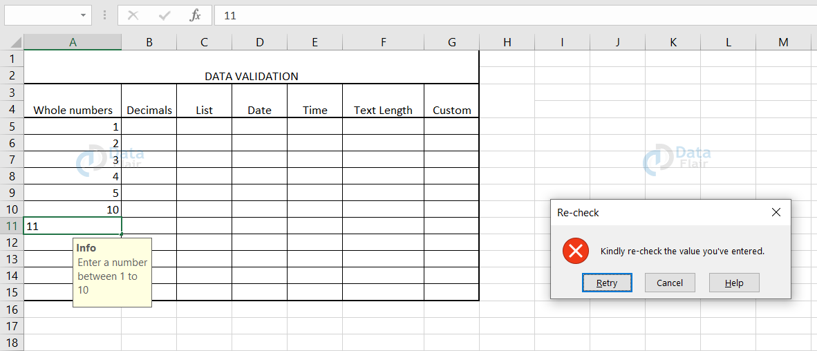
From the sample, you can see that we have chosen the ‘stop’ styling. The title appears has the heading of the box and the message appears inside it.
Press retry to make the changes again in the cell.
Press cancel to close the error alert message.
And if you click on help, then it connects to the online excel help.
Now, let’s look at data validation criteria.
In data validation criteria, we have an allow option with a drop down in it.
This option is where we will choose which type of data fits those cells. There are totally 8 options available in it.
Let’s look at the function it performs when we choose an option from it.
| Allow Option | Performance | Example |
| Any Value | There are no restrictions for these cells. Enter any value. | Decimal, Data, Whole number.. |
| Whole Number | Enter only whole numbers in these cells. | 10,100,10000, 23 |
| Decimal | Enter only decimal numbers in these cells. | 1.1, 2.3, 5.4 |
| List | Enter value from the list in these cells. | Picking a value from the list. If you have a list of 3 countries named India, US, UK. You can pick a value only from it. |
| Date | Enter a value in the date format. | 31-3-2021 |
| Time | Enter a value in the time format. | 03:01:00 |
| Text Length | Enter a text between the length allotted in these cells. | If the text length minimum value is 2 and maximum value is 10, then you have to type a text in between these values like ‘DataFlair’ |
| Custom | Create your own formula | If the custom is set up like the maximum value is 500 and if you enter 501 in the cell. Then, it pops with the error alert message. |
These are the options that are available for the allow label.
We have another component to consider before proceeding with the data validation and that is the data label in the box. It also has a dropdown box from which you have to pick an option to apply for our cells.
Note: To the option ‘Any value’ and ‘Custom’ in the allow label will not require these proceedings. But other options from allow criteria should fill this to apply data validation for the cells.
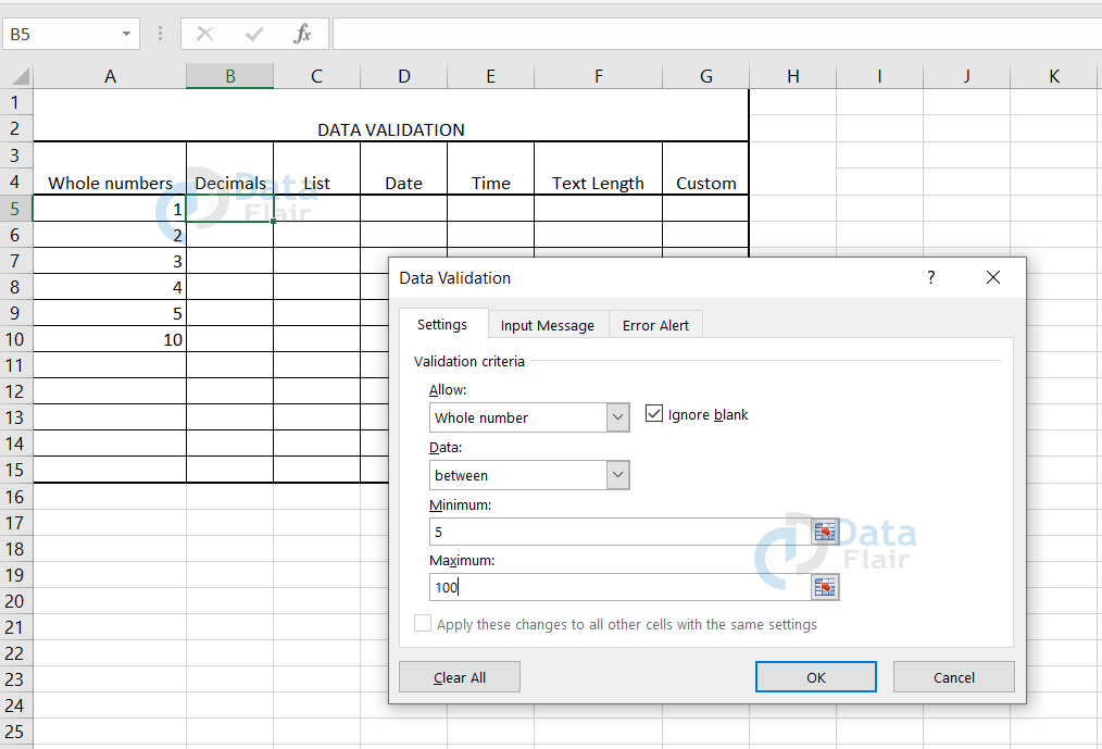
There is always a maximum and minimum value to be filled in the box. Maximum value is the limit that you have to provide for the cell until which it can accept as maximum in those particular cells. Minimum value is the limit from where the cell can accept the value into the cell.
Before entering into a sample, let’s look at data options also.
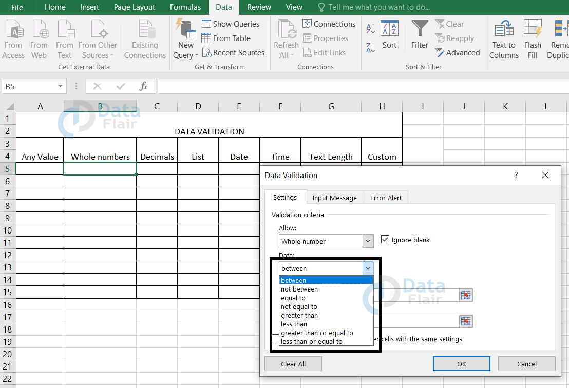
Let’s have a glance at the options available for the data. It contains comparison operators and logical operators in it.
| Data | Minimum | Maximum | Explanation | Example |
| Between | 5 | 10 | Enter a value between 5 to 10. | 7 |
| Not between | 5 | 10 | Enter a value that is not between 5 and 10. | 11 |
| Equal to | – | – | You will not have maximum and minimum value for this option. Instead you have to fill a value in the box. | If you give value =5, then you can enter only 5 in the cells that fall under this criteria. |
| Not equal to | – | – | You will not have maximum and minimum value for this option. Instead you have to fill a value in the box. | Value = 5. Then enter any whole number other than 5. |
| Greater than | 5 | – | You will not have a maximum value here because the condition checks whether it satisfies the minimum criteria only. | Enter a value greater than 5 like 100, 8. |
| Less than | – | 10 | You will not have a minimum value here because the condition checks whether it falls below the maximum value only. | Enter a value less than 10 like 3, 4, 6. |
| Greater than or equal to | 5 | – | You will not have a maximum value here because the condition checks whether it is greater than or equal to the minimum value. | Enter a value greater than or equal to 5 like 5, 6. |
| Less than or equal to | – | 10 | You will not have a minimum value here because the condition checks whether it falls below or equal to the maximum value only. | Enter a value less than or equal to 10 like 9,10. |
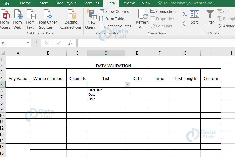
Now, let’s have a look at the sample to understand data validation clearly.
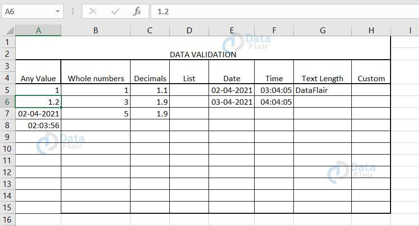
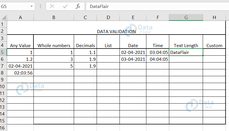
In this sample, we can see that under any value criteria, we can enter any value as there are no restrictions.
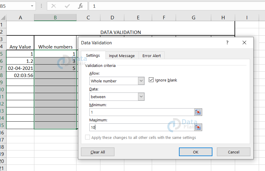
For the whole numbers, I have set the condition as the value should be between 1 and 10. So, if the user enters a value below or above the condition, then an error alert message pops up.
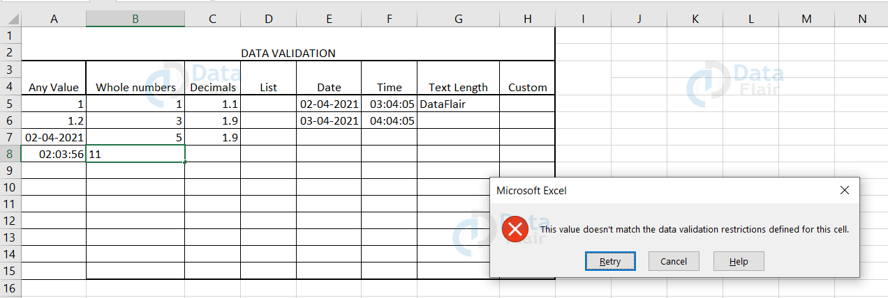
When I tried to enter a value above 10, then the error alert message popped up.
This is how the data validation works for every criteria.
From the sample, we can understand that we have to enter a value that satisfies the condition.
In the sample, for the text length, we have set the minimum and maximum value of the characters. So, when we enter a text, the length of the string should be more than the minimum value but less than the maximum value.
Let’s look at the List criteria in the data validation
List criteria helps the user to pick a value from the source provided. It is also called as dependent lists as the data are dependent on the source.
There are two ways to set up the source. One way to do is:
Typing the drop down list in the source bar.
1: Click on the data tab. Choose data validation from the ribbon.
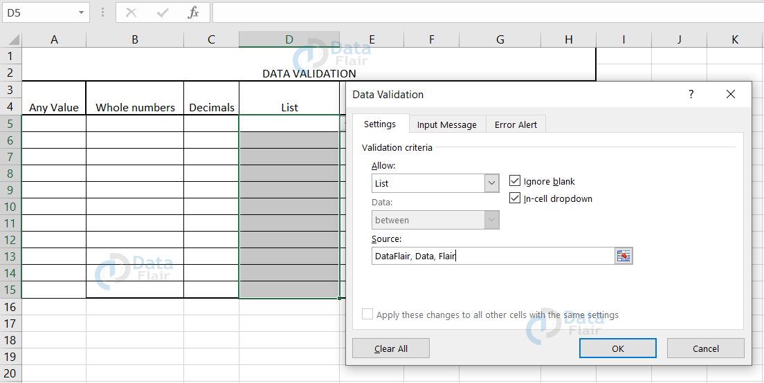
2: Once, the data validation box appears, click on the list from the drop down of the allow label.
3: In the source label, we can fill the data that should appear in the list drop down box.
Note: When you wanted to enter more than one value, then separate it with a comma.
4: Then press OK.
After following the steps, we can see a dropdown option in the list validated cells.
The options that we provided in the source are visible here in the drop down list. Hence, the user enters a value one among the list.
This method will suit fine, only until the source options we provide are less or if we have more data that should appear in the list then typing each option in the source is going to be time consuming. So in order to overcome that issue, we have another method to update the list.
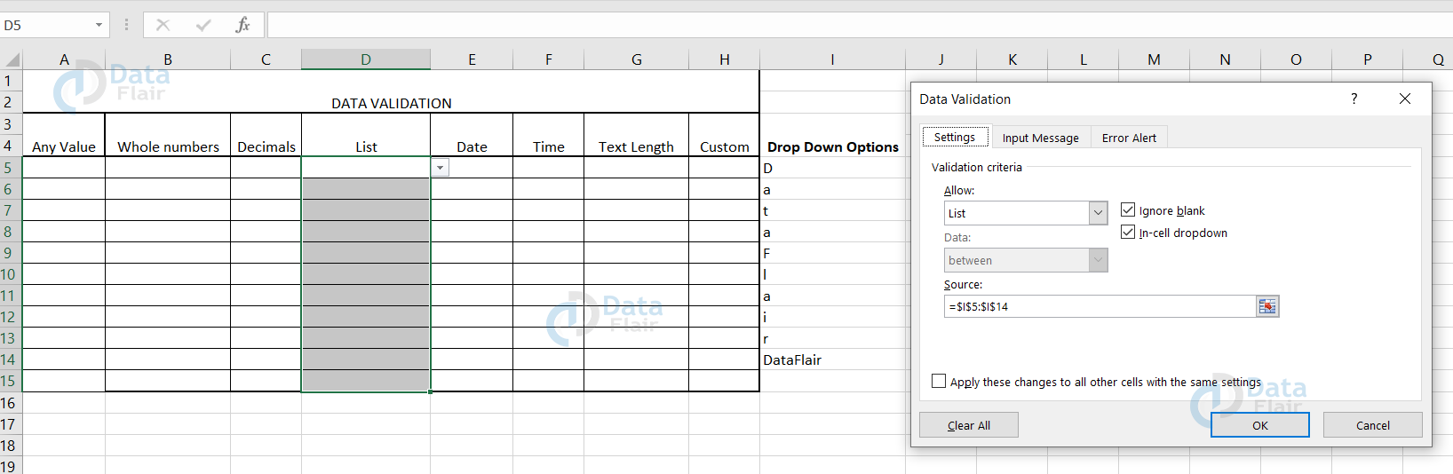
The other method is providing the list as the value of the other cells.
To do so, follow the steps:
1: Click on the data tab.
2: Once the data validation box appears, click on the list from the drop down of the allow label.
3: In the source label, we can fill it out by entering it as the cell number from where to where.
Note: If we are not sure about the cell number, then we can just drag the cells which all should appear in the drop down.
4: Then, click OK.
Let’s have a look at how this type of list works.
From the sample, we can see that I5 to I14 cells are the source provided to the list.
The advantage of having the source list as the cell numbers is that we can also update the list whenever it’s required.
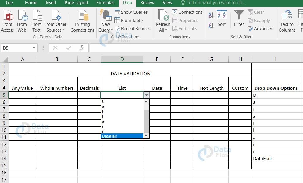
The dropdown options are from the cell I5 to I14.
Custom Data Validation in Excel
In this custom data validation, we can set up the formula as per the requirement.
To set up the custom data validation, follow the steps:
1: Go to Data tab and click on the data validation option from the drop down list.
2: Choose the criteria as custom.
3: A box appears with the data asking for the formula, type the formula and press ok.
Let’s see an example to have a clear understanding of how it works:
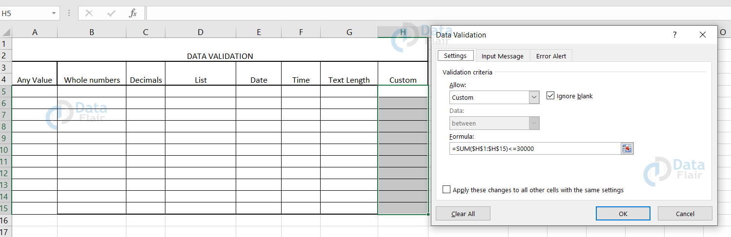
In this sample, I have set the formula as ‘sum($H$1:$H$15)<=30000’ which means if the data exceeds 30000 then the error alert message pops up.
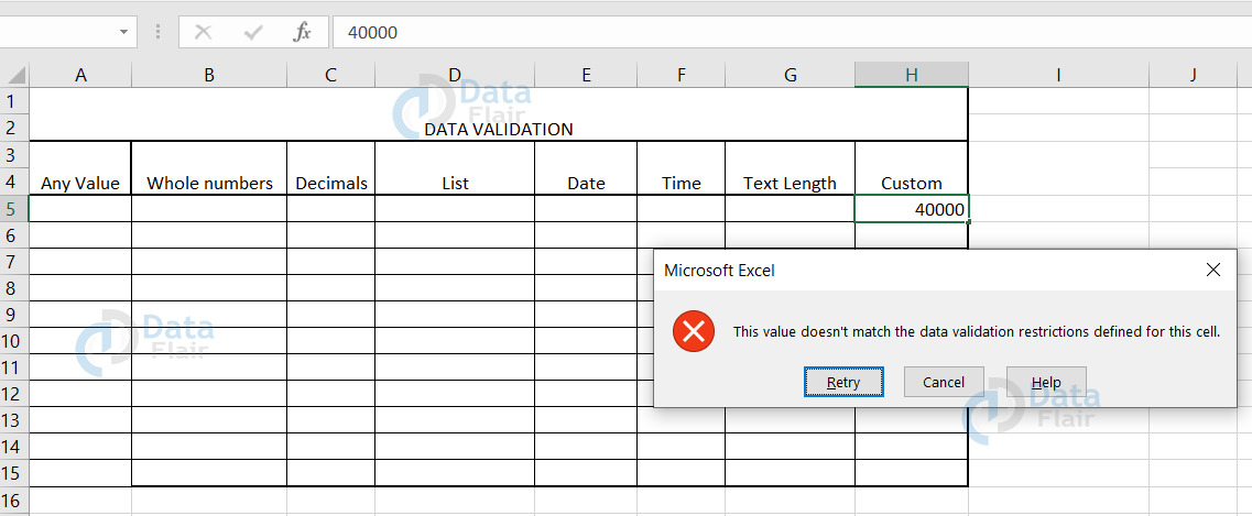
When we tried to enter the value more than 30000, the error alert message popped up.
Therefore, the main advantage of custom data validation is that we can set up the formula as per our convenience.
Circle Invalid Data in Excel
To circle the invalid data, follow the steps:
1: Enter the dataset.
2: Apply the data validation as per the requirement.
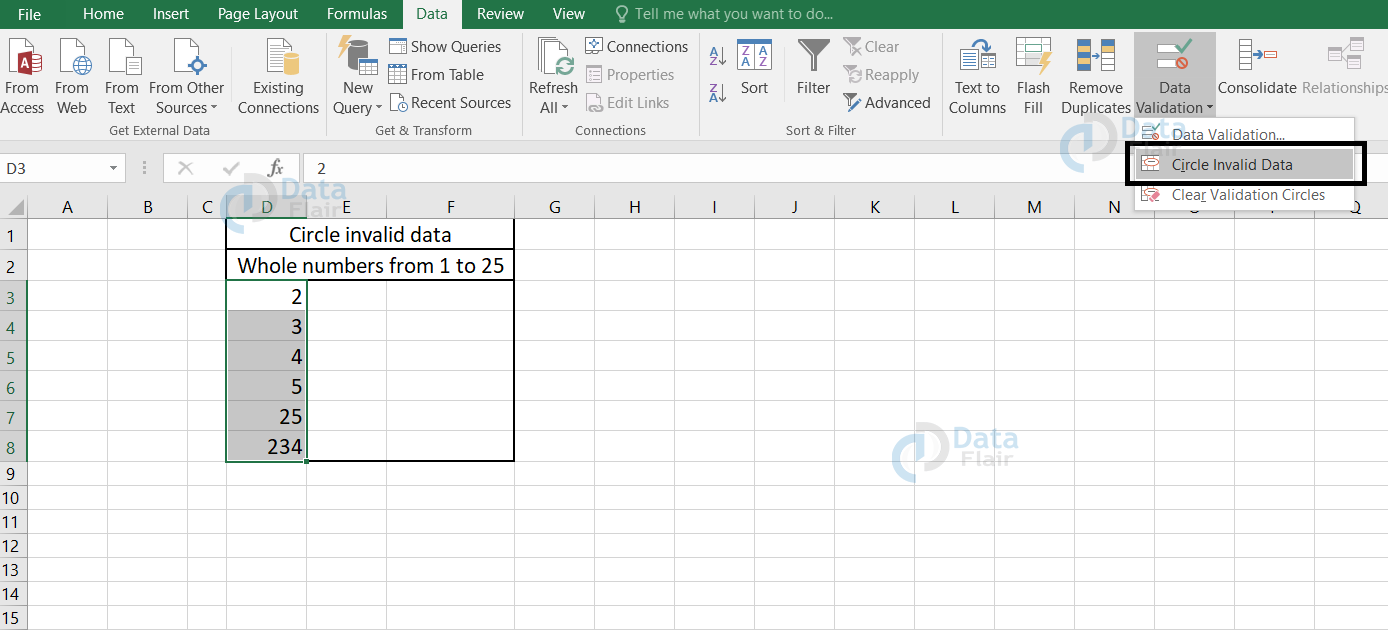
3: Click on the data tab and choose circle invalid data from the ribbon.
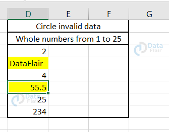
Now, let’s look at a sample:
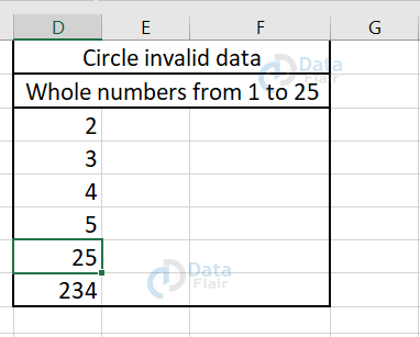
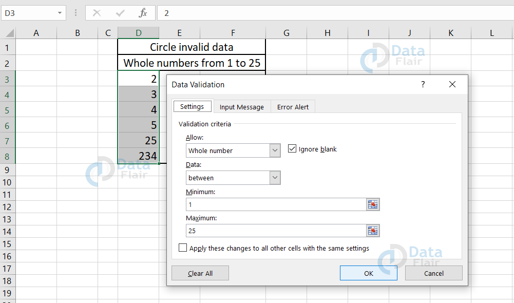
For these cells, we have given the condition that only whole numbers between 1 to 25 should be considered as data validated.
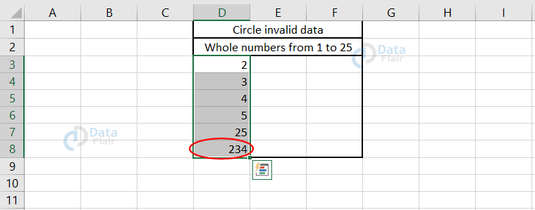
In the above sample, the cells validate only the whole numbers from 1 to 25. But then, there is a whole number of 234 in the D8 cell. This is an invalid data which does not satisfy the criteria. Hence, when we apply circle invalid data, the invalid data cells are circled.
Clear Validation Circles in Excel
When you click on the clear validation circles option, it clears the circle in the spreadsheet.
To apply clear validation circles, follow the steps:
1: Click on the data tab menu.
2: Choose the clear validation circles option from it.
Let’s have a look at the sample for better understanding:
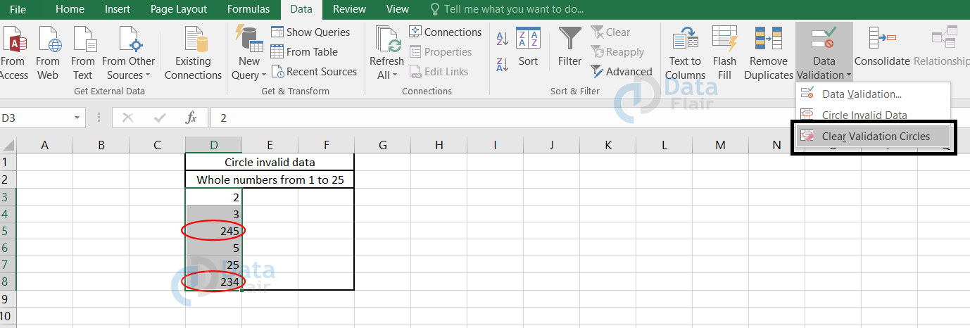
Here, the A5 and A8 cells are invalid as they dont satisfy the criteria. In order to remove the circles from the spreadsheet, click on the clear validation circles.
Once you click on “clear validation circles”, the circles are removed from the spreadsheet.
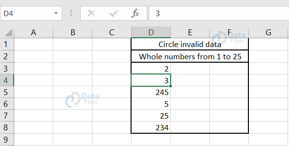
From the sample, we can observe that the circles in the cells are removed.
ClearAll in Excel
When you wanted to remove the data validation on the cells, then click on the “Clear All” option from the box.
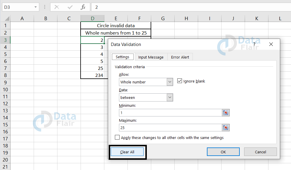
The data validation doesn’t work anymore for those cells.
Hope you see that the text and decimal value are added which means the data validation applied is removed on those cells.
Checking Data Validated cells in Excel
In order to know to which all cells, the data validation is being applied, follow the steps:
1: Click on the Find & Select options dropdown.
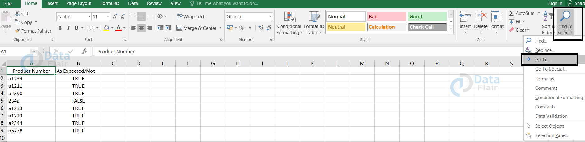
2: Choose the Go To option.
3: A box appears and in that click on the special button.
4: Choose the data validation option in the box
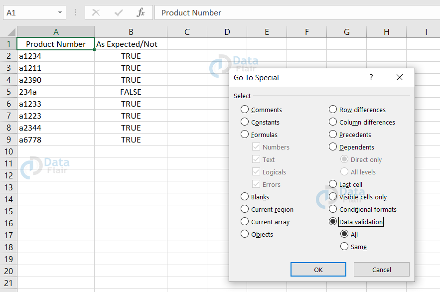
5: Press OK.
From the following above steps, we can know in which all cells the data validation is being applied.
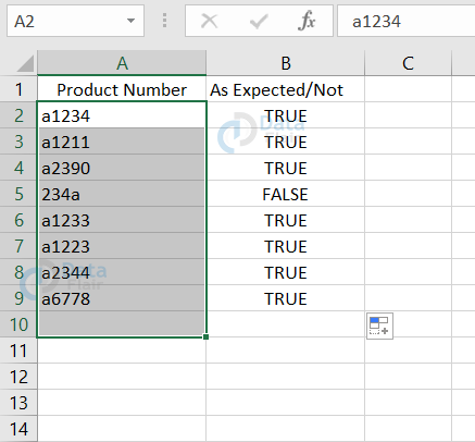
In this, the cells from A2 to A10 are data validated cells.
Limitation in Data Validation in Excel
- Data validation helps the user to set the rule for the cells in the spreadsheet.
- It helps in controlling the value that enters the cell.
- But if the data which are not validated are replaced on the data validated cells, then the data validation will not be applied since the cells are copied and pasted.
Let’s have a look at the sample:
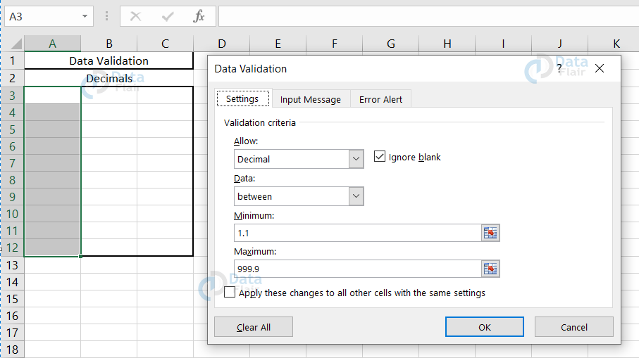
From the above image, we can understand that the cells from A3 to A12 allow only decimal values from 1.1 to 999.9.
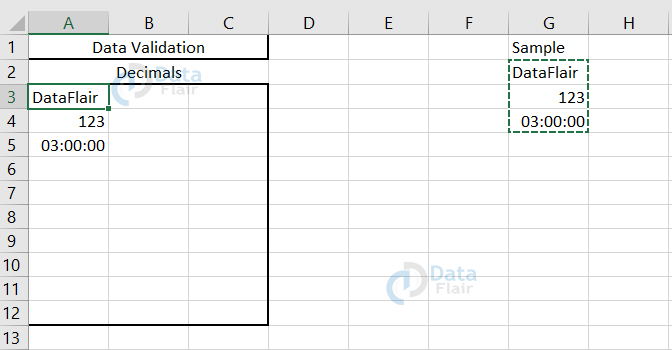
But when the user copies and pastes the values, the data validation applied didn’t restrict but it accepted the values as such. This means that the data validation doesn’t work when the cells are copy-pasted.
Troubleshooting Formulas in Excel
The formulas that return errors are ignored in data validation. In order to check whether the values that are entered in the cells are as per the requirement of the owner, then we can set up the dummy formulas.
Let’s see an example to understand this:
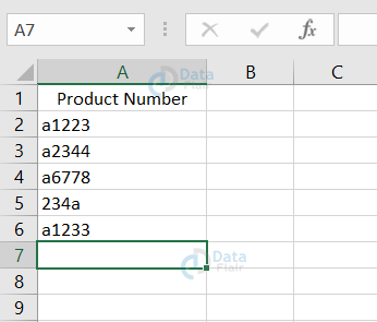
In the above sample, the product number is being noted down. The data validation applied here is text length between 4 to 6. But then, the user didn’t mention how many numbers and letters should be there in the string.
In order to check that, let’s apply a dummy formula.
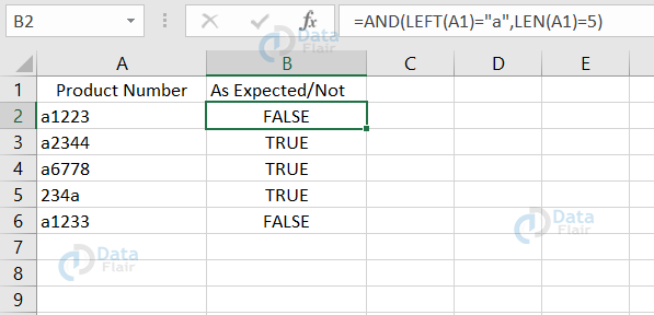
In the above sample, we are checking whether the product number starts with an “A” and the length is 5. If this condition is met, then the formula returns true or else false. Hence, this is how we can test the data validated cells.
Summary
Applying data validation to the cells in the spreadsheet will help in validating the cells. It helps the user to restrict the type of data that enters the cell in the spreadsheet.
Data validation widely helps in setting up limitations of the entry in the cell.
You give me 15 seconds I promise you best tutorials
Please share your happy experience on Google


