Graphs in Data Structure
Learn DSA & Get Ready for MAANG Companies Start Now!!
We use graphs very often in our daily life. Whether it’s going to the office from home or going to a movie with your friends. We use graphs for finding the optimal solution to the problem. In this article, we will learn about types of graphs and how they are useful in deriving the best optimal solution
Graphs
A graph is a non-linear data structure unlike arrays and linked lists. It consists of vertices (nodes) and edges represented by V and E respectively. A graph G can be defined as an ordered set G(V, E) where edges connect the vertices.
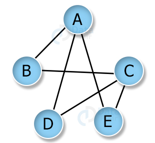
Let us consider a graph G(V, E) with vertices (A, B, C, D, E) and edges ((A,B), (B,C), (C,E), (E,A), (C,D), (A,D)):.
Directed graph and undirected graph
In an undirected graph, the edges are not associated with any direction. In an undirected graph, edges are traversable in both directions. For example, in the above graph, we can traverse E(A, B) from A to B as well as B to A.
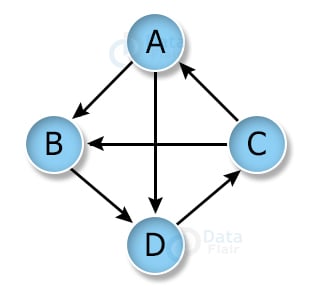
If the edges have a direction as shown below, then it is a directed graph. The E(A, B)is traversable only in the direction of the edge between V(A, B).
Graph terminologies
1. Path: A path is the sequence of nodes that is followed to reach some terminal vertex X from the initial vertex Y.
2. Closed path: A path is a closed path if the initial vertex is the same as the terminal vertex.
3. Simple path: If all the vertices in the graph are distinct (exception V0=Vn), then path P is a closed simple path.
4. Cycle: A cycle is a path that has no repeated edges or vertices except the first and last vertices.
5. Connected graph: In a connected graph each pair of nodes has a path between them i.e. we can reach any vertex by starting from any vertex in the graph. There are no isolated nodes in the connected graph.
6. Complete graph: A complete graph is the one in which each pair of nodes has a direct path between them. A complete graph has n(n-1)/2 edges where n is the number of vertices in the graph.
7. Weighted graph: In a weighted graph, each edge is assigned with a data called weight. The weight of an edge E is given as W(E). Weight must be a positive value that defines the cost of traversing the edge R.
8. Digraph: A directed graph is sometimes referred to as a digraph.
9. Loop: An edge that has the same endpoints is a loop.
10. Adjacent nodes: If two nodes A and B are directly connected via an edge E, then the vertices A and B are adjacent nodes.
11. Degree of the node: A degree of a node is the number of edges associated with that node. A node with degree 0 is an isolated node.
Adjacency matrix
An adjacency matrix is a way of representing graphs in form of a boolean matrix. Consider the graph below:
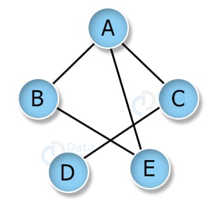
Adjacency matrix for above graph: 1 for edge present and 0 for edge not present.
| A | B | C | D | E | |
| A | 0 | 1 | 1 | 0 | 1 |
| B | 1 | 0 | 0 | 0 | 1 |
| C | 1 | 0 | 0 | 1 | 0 |
| D | 0 | 0 | 1 | 0 | 0 |
| E | 1 | 1 | 0 | 0 | 0 |
Adjacency matrix representation in C
#include <stdio.h>
#define V 4

void init(int arr[][V])
{
  int i, j;
  for (i = 0; i < V; i++)
    for (j = 0; j < V; j++)
      arr[i][j] = 0;
}

void addEdge(int arr[][V], int i, int j)
{
  arr[i][j] = 1;
  arr[j][i] = 1;
}

int main()
{
  int adjMatrix[V][V];

  init(adjMatrix);
  addEdge(adjMatrix, 1, 2);
  addEdge(adjMatrix, 0, 2);
  addEdge(adjMatrix, 3, 0);
  addEdge(adjMatrix, 2, 3);

  int i, j;

  for (i = 0; i < V; i++)
  {
    printf("%d: ", i);
    for (j = 0; j < V; j++)
    {
      printf("%d ", adjMatrix[i][j]);
    }
    printf("\n");
  }

  return 0;
}
Adjacency matrix representation in C++
#include <iostream>
using namespace std;
#define V 4

void init(int arr[][V])
{
  int i, j;
  for (i = 0; i < V; i++)
    for (j = 0; j < V; j++)
      arr[i][j] = 0;
}

void addEdge(int arr[][V], int i, int j)
{
  arr[i][j] = 1;
  arr[j][i] = 1;
}

int main()
{
  int adjMatrix[V][V];

  init(adjMatrix);
  addEdge(adjMatrix, 1, 2);
  addEdge(adjMatrix, 0, 2);
  addEdge(adjMatrix, 3, 0);
  addEdge(adjMatrix, 2, 3);

  int i, j;

  for (i = 0; i < V; i++)
  {
    cout <<  i << ":";
    for (j = 0; j < V; j++)
    {
      cout << " " <<adjMatrix[i][j];
    }
    cout << "\n";
  }

  return 0;
}
Representation of Adjacency matrix in JAVA
public class DSGraph
{
  private boolean adjMatrix[][];
  private int Vertices;

  public DSGraph(int Vertices)
  {
    this.Vertices = Vertices;
    adjMatrix = new boolean[Vertices][Vertices];
  }

  public void addEdge(int i, int j)
  {
    adjMatrix[i][j] = true;
    adjMatrix[j][i] = true;
  }

  public void removeEdge(int i, int j)
  {
    adjMatrix[i][j] = false;
    adjMatrix[j][i] = false;
  }

  public String toString()
  {
    StringBuilder s = new StringBuilder();
    for (int i = 0; i < Vertices; i++)
    {
      s.append(i + ": ");
      for (boolean j : adjMatrix[i])
      {
        s.append((j ? 1 : 0) + " ");
      }
      s.append("\n");
    }
    return s.toString();
  }

  public static void main(String args[])
  {
    DSGraph g = new DSGraph(4);

    g.addEdge(1, 2);
    g.addEdge(0, 2);
    g.addEdge(3, 0);
    g.addEdge(2, 3);

    System.out.print(g.toString());
  }
}
Adjacency matrix representation in Python
class Graph(object):

    def __init__(self, size):
        self.adjMatrix = []
        for i in range(size):
            self.adjMatrix.append([0 for i in range(size)])
        self.size = size

    def addEdge(self, x, y):
        self.adjMatrix[x][y] = 1
        self.adjMatrix[x][y] = 1

    def removeEdge(self, v1, v2):
        self.adjMatrix[x][y] = 0
        self.adjMatrix[x][y] = 0

    def __len__(self):
        return self.size

    def printMatrix(self):
        for row in self.adjMatrix:
            for val in row:
                print('{:4}'.format(val), end="")
            print()


def main():
    g = Graph(5)
    g.addEdge(0, 2)
    g.addEdge(1, 2)
    g.addEdge(3, 0)
    g.addEdge(2, 3)

    g.printMatrix()


if __name__ == '__main__':
    main()
Advantages of an adjacency matrix
1. Operations like adding, removing edges, checking if an edge is present or not between any two vertices are highly time-efficient.
2. Very efficient when the graph is very dense and a large number of edges are present. It can even be represented by using a sparse matrix.
3. Huge matrix operations can be easily performed on modern GPUs.
Disadvantages of an adjacency matrix
1. Adjacency matrices require large memory. If the graph has fewer edges, much of the memory occupied by the matrix is waste.
2. Operations like inEdges and outEdges are expensive when performed on an adjacency matrix.
Adjacency list
Due to the disadvantages of the adjacency matrix, an adjacency list is more preferred in some cases.
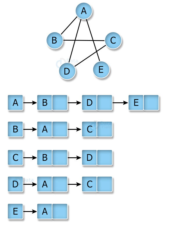
An adjacency list represents a graph in the form of an array of linked lists. The index of the array is vertex and the linked list at that index represents other vertices that form an edge with the index vertex.
Advantages of adjacency lists
1. The adjacency list is highly efficient in storage. For a graph with millions of edges and vertices, adjacency lists are highly beneficial.
Common operations on graph
1. Graph traversal
2. Finding all the paths from one vertex to another
3. Check if the element is present or not in the graph
4. Add and remove nodes and edges in the graph.
Conclusion
Graphs are a non-linear data structure that can be used to model any real-world problem. Graphs are visual tools that make working with very large data easy. Information is easily accessible in graphs. In further articles, we will learn about traversing algorithms and operations on the graphs.
Did we exceed your expectations?
If Yes, share your valuable feedback on Google


