Asymptotic Analysis of Algorithms in Data Structures
Learn DSA & Get Ready for MAANG Companies Start Now!!
Assume your task is to clean your room. Now, what will be the difficulty of the task? It depends on how scattered the room is. If the room is already organized, it will take you no time, and if the room is highly scattered, it might take you hours to arrange it.
So you see, the complexity or difficulty of any task is determined by how much time it takes for its completion. Similarly, it happens in a computer program also. While writing an algorithm, we need to make sure it works fastest with the given resources.
In this article, we will learn what is asymptotic analysis, how to calculate time complexity, what are asymptotic notations, and the time complexity of some frequently used algorithms.
Asymptotic Analysis of Algorithms
The asymptotic analysis defines the mathematical foundation of an algorithm’s run time performance. If there is no input to an algorithm then the algorithm will always work in a constant time.
- Asymptotic analysis is the running time of any process or algorithm in mathematical terms.
- We can calculate the best, average, and worst-case scenarios for an algorithm by using asymptotic analysis.
Basics of asymptotic analysis
In computer programming, the asymptotic analysis tells us the execution time of an algorithm. The lesser the execution time, the better the performance of an algorithm is.
For example, let’s assume we have to add an element at the starting of an array. Since an array is a contiguous memory allocation, we cannot add an element at the first position directly. We need to shift each element to the next position and then only we can add elements at the first position. So we need to traverse the whole array once. The greater the array size, the longer the execution time.
While performing a similar operation on a linked list is comparatively very easy since in a linked list each node is in connection with the next node via a pointer. We can just create a new node and point it to the first node of a linked list. So you can see that adding an element at the first position in a linked list is very much easier as compared to performing a similar operation on an array.
We similarly compare different data structures and select the best possible data structure for an operation. The less the execution time, the higher the performance.
How to find time complexity?
Computing the real running time of a process is not feasible. The time taken for the execution of any process is dependent on the size of the input.
For example, traversing through an array of 5 elements will take less time as compared to traversing through an array of 500 elements. We can observe that time complexity depends on the input size.
Hence, if the input size is ‘n’, then f(n) is a function of ‘n’ denoting the time complexity.
How to calculate f(n) in data structure?
Calculating f(n) value for small programs is easy as compared to bigger programs.
We usually compare data structures by comparing their f(n)values. We also need to find the growth rate of an algorithm because in some cases there is a possibility that for a smaller input size, one data structure is better than the other but when the input data size is large, it’s vice versa.
For example:
Let’s assume a function f(n) = 8n2 +5n+12.
Here n represents the number of instructions executed.
If n=1 :
Percentage of time taken due to 8n2 = (8/(8+5+12))*100 = 32%
Percentage of time taken due to 5n = (5/(8+5+12))*100 = 20%
Percentage of time taken due to 12 = (12/(8+5+12))*100 = 48%
In the above example, we can see that most of the time is taken by ‘12’. But based on only one example we cannot conclude time complexity. We have to calculate the growth factor and then observe the situation as we did in the table below.
| n | 8n2 | 5n | 12 |
| 1 | 32% | 20% | 48% |
| 10 | 92.8% | 5.8% | 1.4% |
| 100 | 99.36% | 0.62% | 0.015% |
| 1000 | 99.93% | 0.06% | ≈ 0 % |
In the above table, we can observe that the 8n2 term is contributing most of the time. It is so much greater than the other two terms that we can ignore those two terms. Therefore, the complexity for this algorithm is :
F(n) = 8n2
This is the approximate time complexity which is very close to the actual result. This measure of approximate time complexity is known as asymptotic complexity.
Here, we are considering the term which takes most of the time and eliminating the unnecessary terms. Though, we’re not calculating the exact running time still it is very close to it.
The time required for the execution of an algorithm is categorized into three types:
- Worst case: the maximum time required for the execution
- Average case: average time taken for the execution.
- Best case: minimum time taken for the execution.
Asymptotic notation
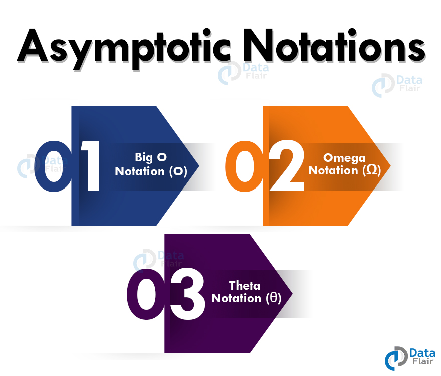
Commonly used asymptotic notation for representing the runtime complexity of an algorithm are:
- Big O notation (O)
- Omega notation (Ω)
- Theta notation (θ)
1. Big O notation (O)
This asymptotic notation measures the performance of an algorithm by providing the order of growth of the function. It provides an upper bound on a function ensuring that the function never grows faster than the upper bound.
It measures the worst-case complexity of the algorithm. Calculates the longest amount of time taken for execution. Hence, it is a formal way to express the upper boundary of an algorithm’s running time.
Let’s analyze the graph below:
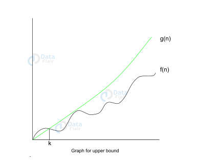
Let f(n), g(n) be two functions, where n ∈ Z+,
f(n) = O(g(n)) [since f(n) is of the order of g(n)].
If there exists constants ‘c’ and ‘k’ such that:
f(n) ≤ c.g(n) for all n≥k
We can conclude that f(n), at no point after n=k, grows faster than g(n). Here, we are calculating the growth rate of the function. This calculates the worst time complexity of f(n).
O(1) example: int arr=new int[10];
This step in any program will execute in O(1) time.
O(n) example: Traversing an array or a linked list. Traversing depends on the size of the array or linked lists.
O(n2) example: Bubble sort algorithm.
2. Omega notation (Ω)
Opposite to big o notation, this asymptotic notation describes the best-case scenario. It is a formal way to present the lower bound of an algorithm running time. This means that this is the minimum time taken for the execution of an algorithm. It is the fastest time that an algorithm can run.
Let’s analyze the below graph :
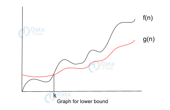
Let f(n), g(n) be two functions, where n ∈ Z+,
f(n) = Ω(g(n)) [since f(n) is of the order of g(n)].
If there exists constants ‘c’ and ‘k’ such that:
f(n) >= c.g(n) for all n≥k and c>0
As you can observe in the above graph that g(n) is the lower bound of the f(n). Hence, this notation gives us the fastest running time. But, we are not interested in the fastest running time. Instead, we are interested in calculating the worst-case scenarios. Because we need to check our algorithm for larger input and what is the worst time that it will take to execute.
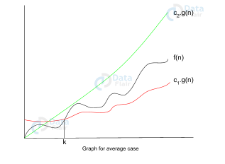
3. Theta notation (θ)
This asymptotic notation describes the average case scenario. An algorithm cannot perform worst or best especially when the problem is a real-world problem. The time complexity fluctuates between best case and worst case and this is given by theta notation (θ) which describes the average case.
Theta notation is mainly used when the value of the worst-case and best-case are the same. It represents both the upper bound and the lower bound of the running time for an algorithm.
Let f(n), g(n) be two functions , where n ∈ Z+,
f(n) = θ(g(n)) [since f(n) is of the order of g(n)].
If there exists constants ‘c’ and ‘k’ such that:
c1.g(n) <= f(n) <= c2.g(n)
Here f(n) has a limitation of an upper bound and a lower bound. The condition f(n)= θg(n) will be true only if it satisfies the above equation. Below is the graphical representation of theta notation is:
Let us see an example for better understanding :
Assume we have to reverse the string: “DATAFLAIR”
Let’s have a look at the traditional Algorithm for it :
Step 1: Start
Step 2: Declare two variables str1 and str2.
Step 3: Initialize the variable str1 with “DATAFLAIR”
Step 4: Go to the last character of str1
Step 5: Take each character starting from the end, from str1, and append it to str2.
Step 6: Print str2
Step 7: Stop
In the above algorithm, each time step 5 is executed, a new string is created. It does not append it to the original string. Instead, it creates a new string and assigns it to str2 every time. Thus the complexity for this algorithm is O(n2).
But in JAVA, we have the StringBuffer.reverse() function which reserves room for characters without reallocation. Therefore, reversing a string using StringBuffer.reverse() in JAVA is possible only in O(1).
What is the need for Asymptotic analysis?
Let’s compare linear search and binary search algorithms:
Execution time for linear search: a*n
Execution time for binary search: b*(log n)
a,b => contents, n=> input size.
Since n > log n, linear search takes more time to execute than binary search. But what if Linear search is executed on a very faster system.
| Machine A (Linear Search ) | Machine B (Binary Search) |
| 10^9 instructions per second | 10^6 instructions per second |
| For n=1000: Execution time = n / 109 = 1000 / 109 = 10-6 seconds (FASTER) | For n = 1000: Execution time = log n / 106 = log 1000 / 106 = 3 * 10-6 seconds (SLOWER) |
| For n=1000000 ( 1 million ): Execution time = n / 109 = 1000000 / 109 = 10-3 seconds (SLOWER) | For n=1000000 ( 1 million ): Execution time = log n / 109 = log 1000000 / 109 = 5 * 10-9 seconds (FASTER) |
We can see that linear search works better for a shorter input but binary search works better for larger input even though the linear search is run on a faster system. This is why we need asymptotic analysis so that we can calculate time complexity as close to the real value as possible.
Why have three different notations?
Let’s try to find out the complexity of the linear search algorithm. Suppose you want to search an element in an array using the linear search algorithm. In a linear search algorithm, the search element is compared to each element of the array.
If the element is found at the first position itself, it is a best-case and the program will take the least time for execution. The complexity will be Ω(1). If the element is found at the last position, it will be the worst-case scenario and the program will take maximum time for execution. Its time complexity will be O(n).
The average case complexity is between worst case and best case so it becomes θ(n/1). Since we can ignore the constant terms in asymptotic notations the average-case complexity will be θ(n).
Some more Asymptotic Notation in Data Structures
Following are 2 more asymptotic notation used:
1. Little ‘ο’ notation
This notation provides a loose upper bound on a function. Little order is an estimate of the order of growth, unlike big O, which is an actual order of growth.
Let’s analyze the graph below:
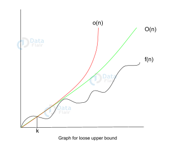
Let f(n), g(n) be two functions, where n ∈ Z+,
f(n) = o(g(n)) [since f(n) is of the order of g(n)].
If for any constant ‘c’ > 0 , there exists a constant ‘k’ >1, such that:
0 ≤ f(n) ≤ c.g(n).
We can conclude that f(n), at no point after n=k, grows faster than g(n). Here, we are calculating the approximate growth rate of the function.
2. Little ω notation
This notation provides a loose lower bound on a function. Little order is an estimate of the order of growth, unlike big Ω, which is the actual order of growth.
Let’s analyze the graph:
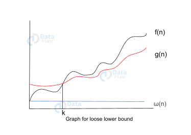
Let f(n), g(n) be two functions, where n ∈ Z+,
f(n) = ω(g(n)) [since f(n) is of the order of g(n)].
If for any constant ‘c’ > 0 , there exists a constant ‘k’ >=1, such that:
f(n) > c.g(n) >=0, for every integer n>=k.
Advantages of asymptotic notations
1. Asymptotic analysis is the best and efficient way of analyzing algorithms with actual runtime inputs.
2. Analyzing algorithms manually is not feasible as the performance of the algorithms changes with the input change.
Also, the algorithm’s performance changes with different machines. Therefore, having a mathematical representation that gives us the actual insight of the maximum and minimum time taken for execution is better.
3. We can represent the upper bound or lower bound of execution time in the form of mathematical equations.
4. Asymptotic analysis of algorithms helps us in performing our task with the best efficiency and fewer efforts.
Commonly used asymptotic notations
| Type | Big O notation |
| Constant | O(1) |
| Linear | O(n) |
| Logarithmic | O(log n) |
| N log n | O(n log(n)) |
| exponential | 2O(n) |
| cubic | O(n3) |
| polynomial | nO(1) |
| quadratic | O(n2) |
Run time performance of the above complexities are :
O(1) < O(log n) < O(n) < O(n log n) < O(n2) < O (n3)< O(2n) < O(n!)
Time Complexity of some frequently used algorithms
Below is the list of some commonly used algorithms and their worst-case complexities. We will learn how to calculate these complexities in future articles.
| Algorithm | Worst Case Time Complexity |
| Linear search | O(n) |
| Binary Search | O(log n) |
| Selection sort | O(n2) |
| Bubble Sort | O(n2) |
| Insertion sort | O(n2) |
| Merge Sort | O(n log(n)) |
| Quicksort | O(n2) |
| Bucket sort | O(n2) |
| Radix sort | O(nk) |
Conclusion
In this article, we learned what are asymptotic notations. Now we are aware of how to calculate asymptotic notations and time complexities for different kinds of algorithms.
We also observed the mathematical graphs and proofs for best case, worst case, and average case scenarios. We will see detailed derivations of the complexities for the above-mentioned algorithms in future articles.
Did you know we work 24x7 to provide you best tutorials
Please encourage us - write a review on Google


