Support Vector Machines Tutorial – Learn to implement SVM in Python

Support Vector Machines Tutorial – I am trying to make it a comprehensive plus interactive tutorial, so that you can understand the concepts of SVM easily.

A few days ago, I met a child whose father was buying fruits from a fruitseller. That child wanted to eat strawberry but got confused between the two same looking fruits. After noticing for a while he understands which one is Strawberry and picks one from the basket. Same as that child, support vector machines work. It looks at data and sorts it into one of the two categories.

Still confused? Read the article below to understand SVM in detail with lots of examples.

Introduction to Support Vector Machines

SVMs are the most popular algorithm for classification in machine learning algorithms. Their mathematical background is quintessential in building the foundational block for the geometrical distinction between the two classes. We will see how Support vector machines work by observing their implementation in Python and finally, we will look at some of the important applications.

What is SVM?

Support Vector Machines are a type of supervised machine learning algorithm that provides analysis of data for classification and regression analysis. While they can be used for regression, SVM is mostly used for classification. We carry out plotting in the n-dimensional space. Value of each feature is also the value of the specific coordinate. Then, we find the ideal hyperplane that differentiates between the two classes.

These support vectors are the coordinate representations of individual observation. It is a frontier method for segregating the two classes.

Don’t forget to check DataFlair’s latest tutorial on Machine Learning Clustering

How does SVM work?

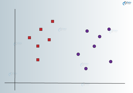
The basic principle behind the working of Support vector machines is simple – Create a hyperplane that separates the dataset into classes. Let us start with a sample problem. Suppose that for a given dataset, you have to classify red triangles from blue circles. Your goal is to create a line that classifies the data into two classes, creating a distinction between red triangles and blue circles.

While one can hypothesize a clear line that separates the two classes, there can be many lines that can do this job. Therefore, there is not a single line that you can agree on which can perform this task. Let us visualize some of the lines that can differentiate between the two classes as follows –

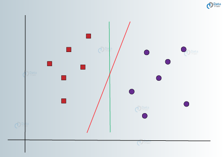
In the above visualizations, we have a green line and a red line. Which one do you think would better differentiate the data into two classes? If you choose the red line, then it is the ideal line that partitions the two classes properly. However, we still have not concretized the fact that it is the universal line that would classify our data most efficiently.

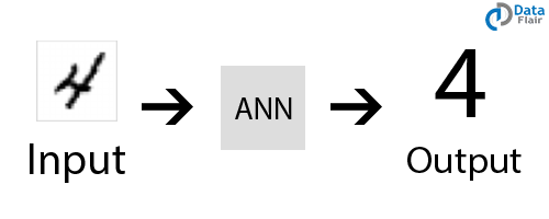
At this point, you can’t miss learning about Artificial Neural Networks

The green line cannot be the ideal line as it lies too close to the red class. Therefore, it does not provide a proper generalization which is our end goal.

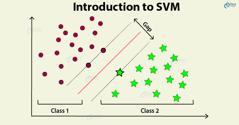
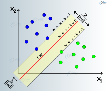
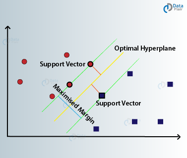
According to SVM, we have to find the points that lie closest to both the classes. These points are known as support vectors. In the next step, we find the proximity between our dividing plane and the support vectors. The distance between the points and the dividing line is known as margin. The aim of an SVM algorithm is to maximize this very margin. When the margin reaches its maximum, the hyperplane becomes the optimal one.

The SVM model tries to enlarge the distance between the two classes by creating a well-defined decision boundary. In the above case, our hyperplane divided the data. While our data was in 2 dimensions, the hyperplane was of 1 dimension. For higher dimensions, say, an n-dimensional Euclidean Space, we have an n-1 dimensional subset that divides the space into two disconnected components.

Next in this SVM Tutorial, we will see implementing SVM in Python. So, before moving on I recommend revise your Python Concepts. 

How to implement SVM in Python?

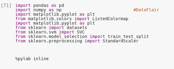
In the first step, we will import the important libraries that we will be using in the implementation of SVM in our project.

Code:

import pandas as pd
import numpy as np                            #DataFlair
import matplotlib.pyplot as plt
from matplotlib.colors import ListedColormap
import matplotlib.pyplot as plt
from sklearn import datasets
from sklearn.svm import SVC
from sklearn.model_selection import train_test_split
from sklearn.preprocessing import StandardScaler

%pylab inline

Screenshot:

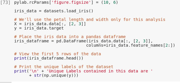
In the second step of implementation of SVM in Python, we will use the iris dataset that is available with the load_iris() method. We will only make use of the petal length and width in this analysis.

Code:

pylab.rcParams['figure.figsize'] = (10, 6)

iris_data = datasets.load_iris()

# We'll use the petal length and width only for this analysis
X = iris_data.data[:, [2, 3]]
y = iris_data.target

# Input the iris data into the pandas dataframe
iris_dataframe = pd.DataFrame(iris_data.data[:, [2, 3]],
                  columns=iris_data.feature_names[2:])

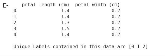
# View the first 5 rows of the data
print(iris_dataframe.head())

# Print the unique labels of the dataset
print('\n' + 'Unique Labels contained in this data are '
     + str(np.unique(y)))

Screenshot:

ALERT!! You are missing something important – Don’t forget to practice the latest machine learning projects. Here is one for you – Credit Card Fraud Detection using Machine Learning 

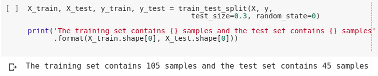
In the next step, we will split our data into training and test set using the train_test_split() function as follows –

Code:

X_train, X_test, y_train, y_test = train_test_split(X, y, test_size=0.3, random_state=0)

print('The training set contains {} samples and the test set contains {} samples'.format(X_train.shape[0], X_test.shape[0]))

Screenshot:

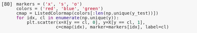
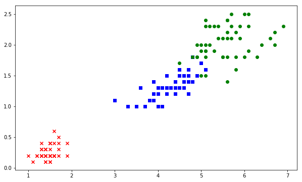
Let us now visualize our data. We observe that one of the classes is linearly separable.

Code:

markers = ('x', 's', 'o')
colors = ('red', 'blue', 'green')
cmap = ListedColormap(colors[:len(np.unique(y_test))])
for idx, cl in enumerate(np.unique(y)):
    plt.scatter(x=X[y == cl, 0], y=X[y == cl, 1],
           c=cmap(idx), marker=markers[idx], label=cl)

Screenshot:

Output:

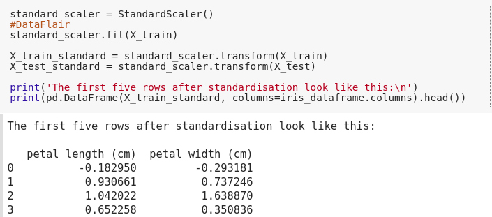
Then, we will perform scaling on our data. Scaling will ensure that all of our data-values lie on a common range such that there are no extreme values.

Code:

standard_scaler = StandardScaler()
#DataFlair
standard_scaler.fit(X_train)

X_train_standard = standard_scaler.transform(X_train)
X_test_standard = standard_scaler.transform(X_test)

print('The first five rows after standardisation look like this:\n')
print(pd.DataFrame(X_train_standard, columns=iris_dataframe.columns).head())

Output Screenshot:

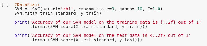
After we have pre-processed our data, the next step is the implementation of the SVM model as follows. We will make use of the SVC function provided to us by the sklearn library. In this instance, we will select our kernel as ‘rbf’.

Code:

#DataFlair
SVM = SVC(kernel='rbf', random_state=0, gamma=.10, C=1.0)
SVM.fit(X_train_standard, y_train)

print('Accuracy of our SVM model on the training data is {:.2f} out of 1'.format(SVM.score(X_train_standard, y_train)))

print('Accuracy of our SVM model on the test data is {:.2f} out of 1'.format(SVM.score(X_test_standard, y_test)))

Screenshot:

DataFlair’s Recommendation – Customer Segmentation using R and Machine Learning

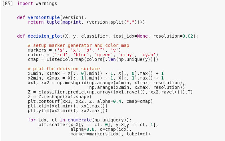
After we have achieved our accuracy, the best course of action would be to visualize our SVM model. We can do this by creating a function called decision_plot() and passing values to it as follows –

Code:

import warnings

def versiontuple(version):
   return tuple(map(int, (version.split("."))))

def decision_plot(X, y, classifier, test_idx=None, resolution=0.02):

   # setup marker generator and color map
   markers = ('s', 'x', 'o', '^', 'v')
   colors = ('red', 'blue', 'green', 'gray', 'cyan')
   cmap = ListedColormap(colors[:len(np.unique(y))])

   # plot the decision surface
   x1min, x1max = X[:, 0].min() - 1, X[:, 0].max() + 1
   x2min, x2max = X[:, 1].min() - 1, X[:, 1].max() + 1
   xx1, xx2 = np.meshgrid(np.arange(x1min, x1max, resolution),
                 np.arange(x2min, x2max, resolution))
   Z = classifier.predict(np.array([xx1.ravel(), xx2.ravel()]).T)
   Z = Z.reshape(xx1.shape)
   plt.contourf(xx1, xx2, Z, alpha=0.4, cmap=cmap)
   plt.xlim(xx1.min(), xx1.max())
   plt.ylim(xx2.min(), xx2.max())

   for idx, cl in enumerate(np.unique(y)):
      plt.scatter(x=X[y == cl, 0], y=X[y == cl, 1],
              alpha=0.8, c=cmap(idx),
              marker=markers[idx], label=cl)

Screenshot:

Code:

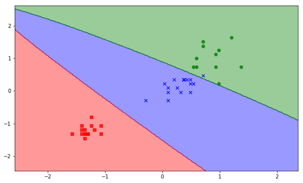
decision_plot(X_test_standard, y_test, SVM)

Screenshot:

Output:

Convolutional Neural Network – You must learn this concept for becoming an expert

Advantages and Disadvantages of Support Vector Machine

Advantages of SVM

• Guaranteed Optimality: Owing to the nature of Convex Optimization, the solution will always be global minimum not a local minimum.
• Abundance of Implementations: We can access it conveniently, be it from Python or Matlab.
• SVM can be used for linearly separable as well as non-linearly separable data. Linearly separable data is the hard margin whereas non-linearly separable data poses a soft margin.
• SVMs provide compliance to the semi-supervised learning models. It can be used in areas where the data is labeled as well as unlabeled. It only requires a condition to the minimization problem which is known as the Transductive SVM.
• Feature Mapping used to be quite a load on the computational complexity of the overall training performance of the model. However, with the help of Kernel Trick, SVM can carry out the feature mapping using simple dot product.

Disadvantages of SVM

• SVM is incapable of handling text structures. This leads to loss of sequential information and thereby, leading to worse performance.
• Vanilla SVM cannot return the probabilistic confidence value that is similar to logistic regression. This does not provide much explanation as confidence of prediction is important in several applications.
• Choice of the kernel is perhaps the biggest limitation of the support vector machine. Considering so many kernels present, it becomes difficult to choose the right one for the data.

Learn everything about Recurrent Neural Networks and its applications

How to Tune SVM Parameters?

Kernel

Kernel in the SVM is responsible for transforming the input data into the required format. Some of the kernels used in SVM are linear, polynomial and radial basis function (RBF). For creating a non-linear hyperplane, we use RBF and Polynomial function. For complex applications, one should use more advanced kernels to separate classes that are nonlinear in nature. With this transformation, one can obtain accurate classifiers.

Regularization

We can maintain regularization by adjusting it in the Scikit-learn’s C parameters. C denotes a penalty parameter representing an error or any form of misclassification. With this misclassification, one can understand how much of the error is actually bearable. Through this, you can nullify the compensation between the misclassified term and the decision boundary. With a smaller C value, we obtain hyperplane of small margin and with a larger C value, we obtain hyperplane of larger value.

Gamma

With a lower value of Gamma will create a loose fit of the training dataset. On the contrary, a high value of gamma will allow the model to get fit more appropriately. A low value of gamma only provides consideration to the nearby points for the calculation of a separate plane whereas the high value of gamma will consider all the data-points to calculate the final separation line.

Applications of SVM

Some of the areas where Support Vector Machines are used are as follows –

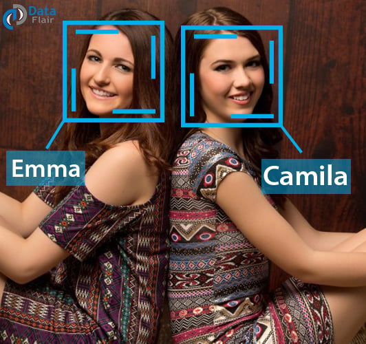
• Face Detection

SVMs are capable of classifying images of persons in an environment by creating a square box that separates the face from the rest.

• Text and hypertext categorization

SVMs can be used for document classification in the sense that it performs the text and hypertext categorization. Based on the score generated, it performs a comparison with the threshold value.

• Bioinformatics

In the field of bioinformatics, SVMs are used for protein and genomic classification. They can classify the genetic structure of the patients based on their biological problems.

• Handwriting recognition

Another area where support vector machines are used for visual recognition is handwriting recognition.

Summary

In this article, we studied about Support Vector Machines. We learned how these SVM algorithms work and also implemented them with a real-life example. We also discussed the various applications of SVMs in our daily lives. Hope now you understand the complete theory of SVM.

What do you want to learn next? Comment below. DataFlair will surely help you.

Till then keep exploring the Machine Learning Tutorials. Happy learning😊