SAP HANA Analytic View – Create Analytic View in 15 Easy Steps

After learning about the Attribute View, let’s move on to understanding the Analytic View. In this lesson, we will first understand the concept behind the Analytic View in SAP HANA.

Then, we will discuss some characteristics of Analytic View and at last, we will proceed to learn how to create an Analytic View in SAP HANA.

What is SAP HANA Analytic View?

The Analytic Views in SAP HANA are one step ahead in terms of complexity as compared to the Attribute View. The Analytic Views are multi-dimensional views involving attributes and measures arranged in a star schema fashion.

In the center lies the fact table, which is a table containing measure columns from the transactional SAP HANA database.

Surrounding this fact table is a different set of attribute tables/views. The attributes or dimensions attached to the fact table making an analytic view provides relevance to the measures in the fact table. Thus, a user can examine data (transactional data) from different perspectives.

For instance, you can have a fact table named Sales linked to four attribute views or dimensions such as Region, Period, Customer, and Product. That is, sales can be analyzed with respect to the regions, customers, years, or products.

The multi-dimensional view created in the analytic view is also representative of OLAP cubes.

Features of SAP HANA Analytic View

Some important features of the analytic view in SAP HANA are:

• Analytic views run start schema queries.
• The measures used in the fact table can be calculated measures or restricted measure.
• You can perform complex calculations and apply aggregation functions (sum, min, max, count etc.) on the data used in the Analytic View.

Steps to Create an Analytic View in SAP HANA

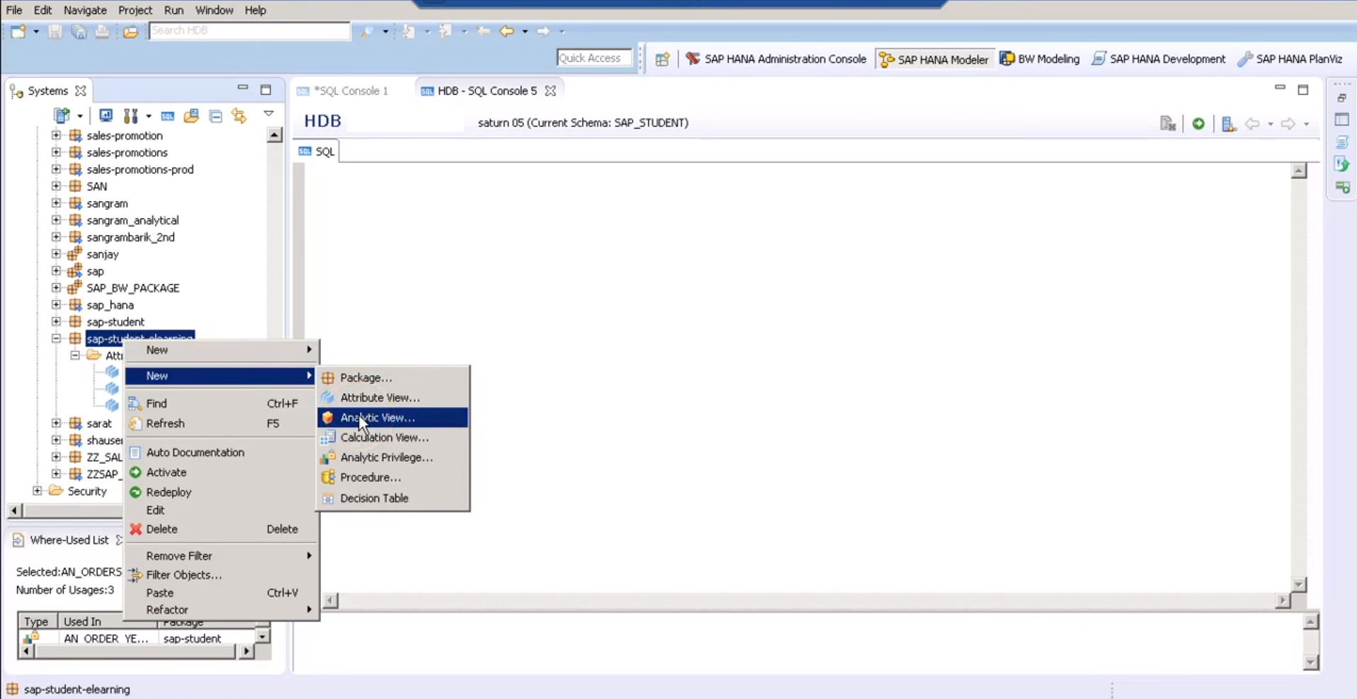
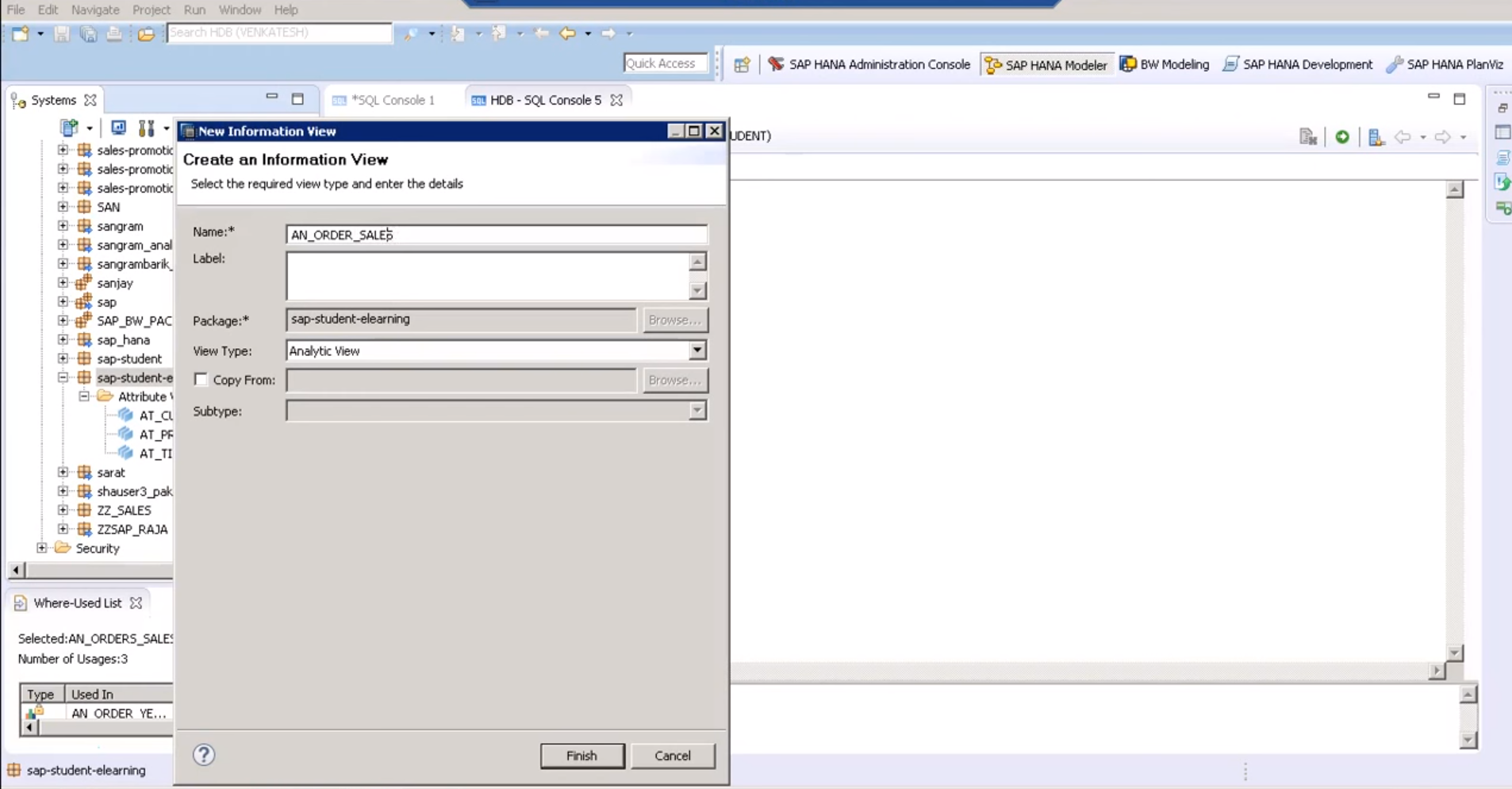
Here are the steps to create an Analytic View in SAP HANA Modeler:

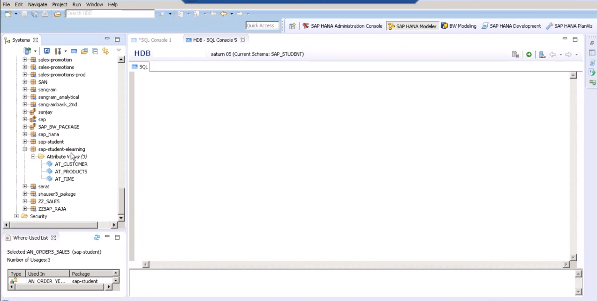
Step 1: Open SAP HANA Modeler perspective in the SAP HANA Studio.

Step 2: Your pre-existing attribute views will be present within a package in the Content node.
Step 3: Right-click on the package for which you need to create an Analytic View in SAP HANA which also contains the attribute views. Click on New and select Analytic view from the drop-down list. Step 4: Enter the technical name of the view and add a description. You can set other properties as well, like view type, subtype etc. Click on Finish.

Step 5: The design view for the analytic view in SAP HANA Modeler opens.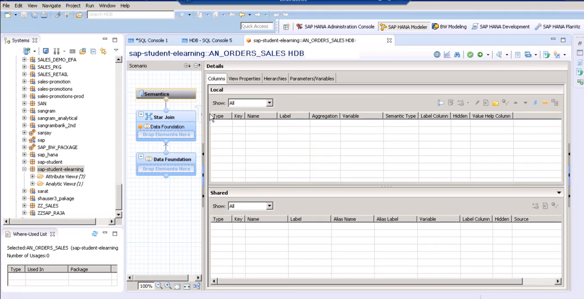 

From the semantics section, you can access the columns, view properties, hierarchies and variables or parameters.

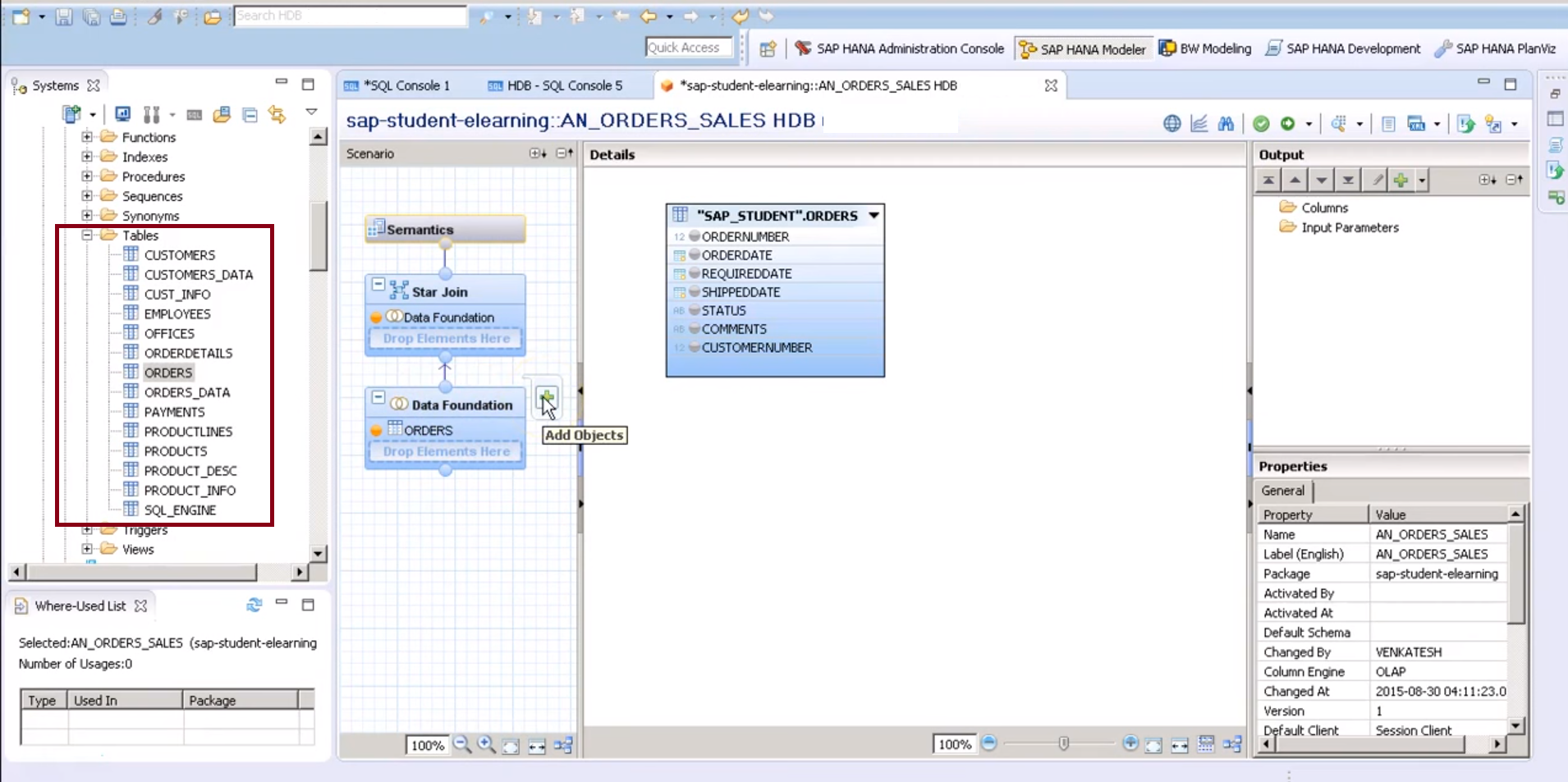
Step 6: Now its time to add tables into the Data foundation. You can add the data tables from the left panel either by dragging and dropping or by searching the table’s name, Add Objects icon.

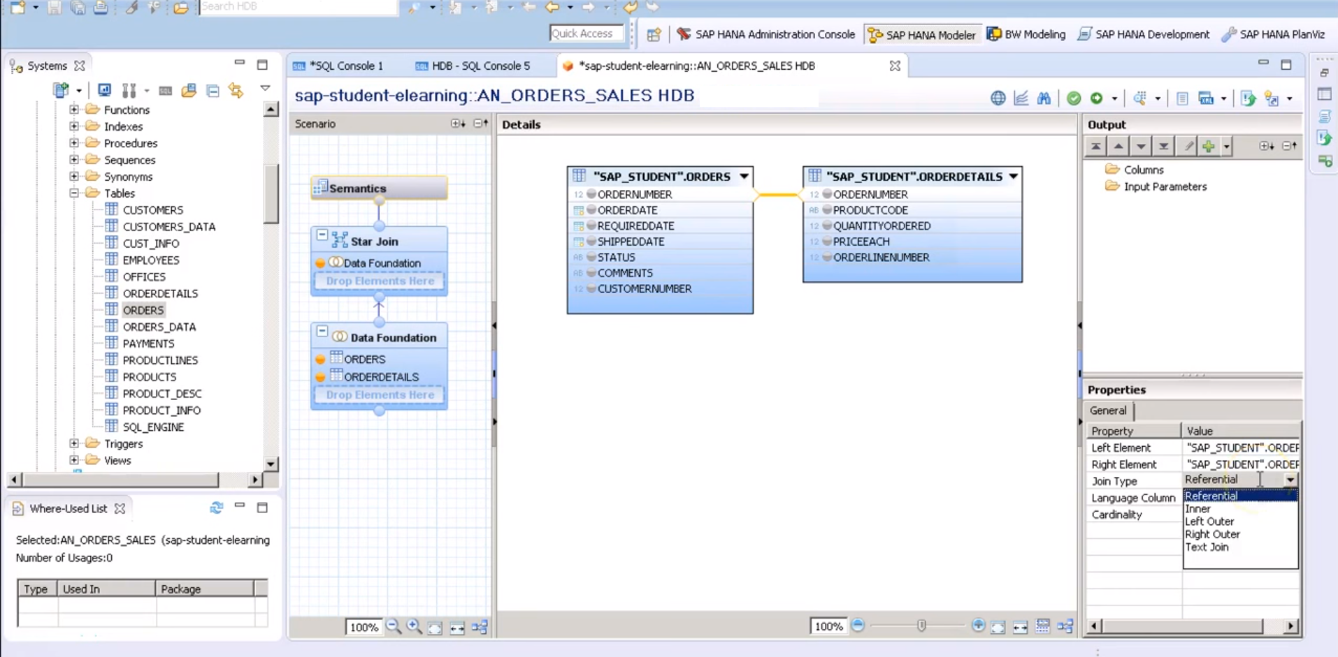
Step 7: If you have more than one table selected, then you need to define a join condition and cardinality. Here, in the image shown below, we have selected join type as inner join and set cardinality as 1: N in the join created two tables ORDERS and ORDERDETAILS.

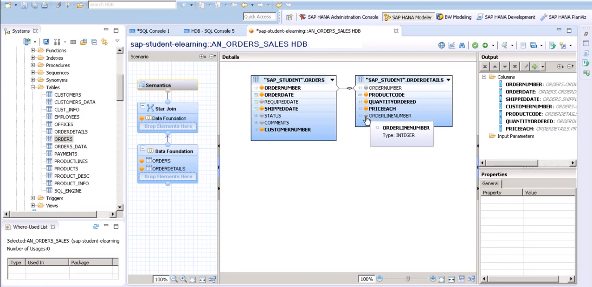
Step 8: Next, we have to select columns for output from both tables by clicking on the grey dots given in front of each column of the table which will turn orange as a sign of being added into the output.

Step 9: Now we will go to the “start join” section to link all the attributes views with the data foundation (fact table). As you can see in the image below, we have selected three attribute views in the Star Join section; AT_CUSTOMER, AT_PRODUCTS and AT_TIME.

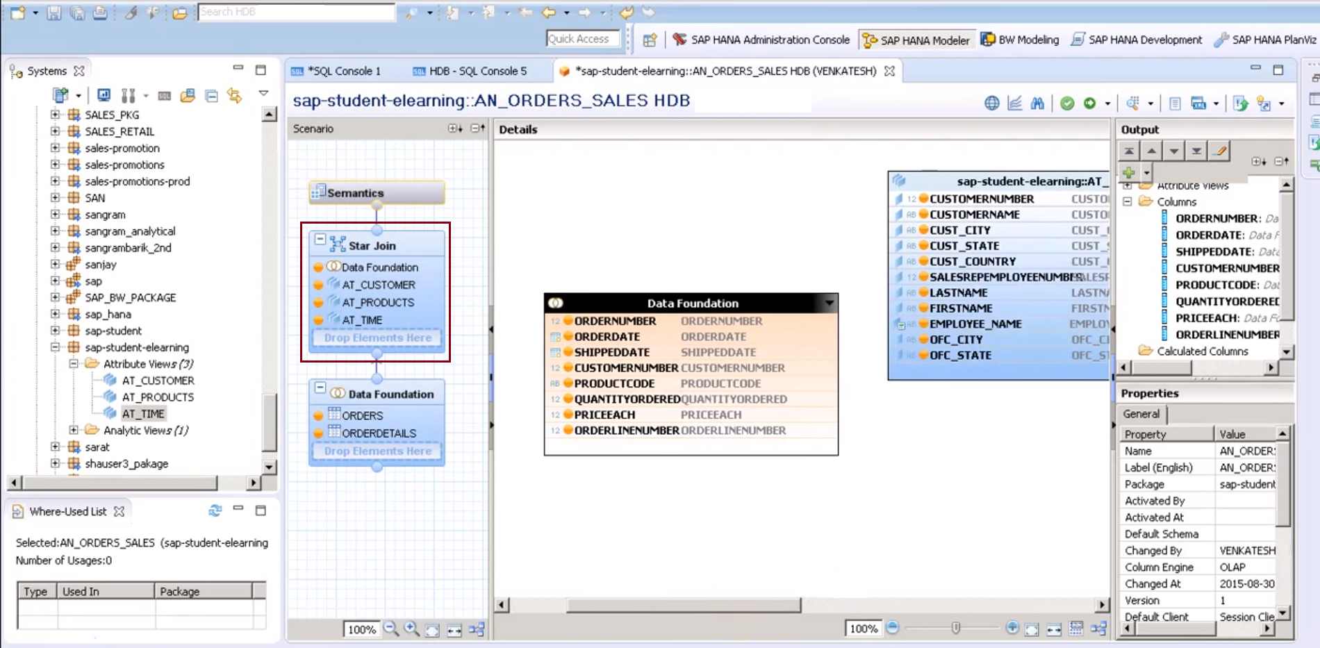
Three separate tables for the three attribute views will get add in the editor pane.

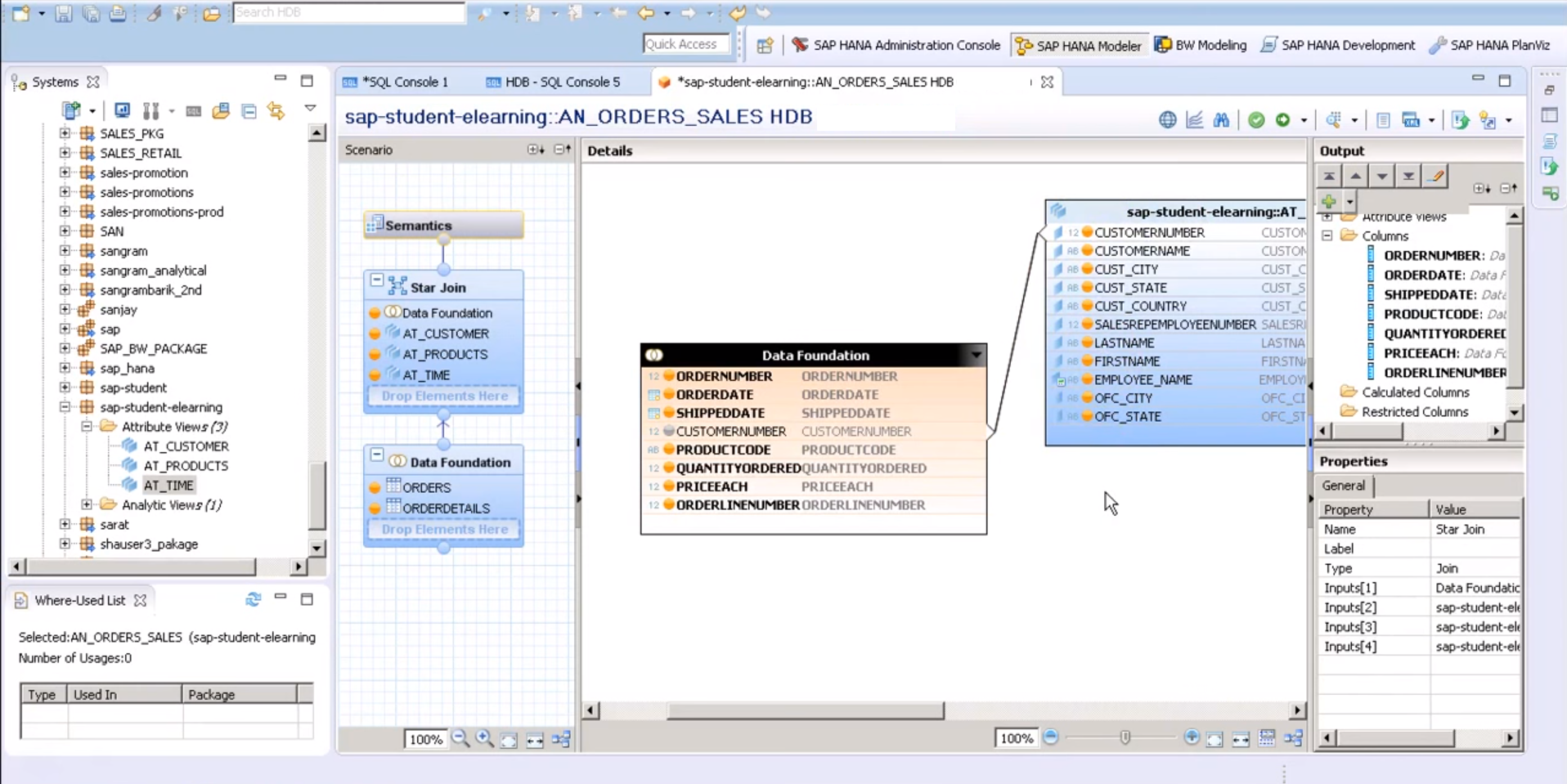
Step 10: We will join the fact table with the attribute view table with common columns, as shown in the image below. We have joined the two tables (fact table and attribute view) with the column CUSTOMERNUMBER.
Also, we have defined the join type as an outer join.

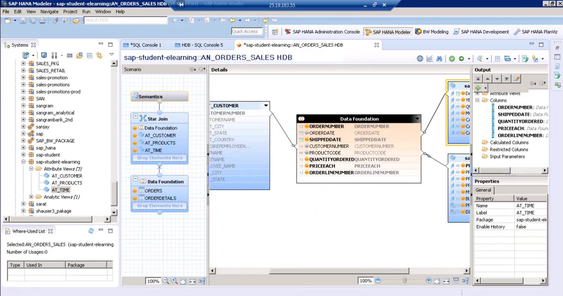
Step 11: We will join the two other attribute tables with the fact table in the same way. This will form a star schema like structure of tables.
Step 12: Next, we’ll define measures and dimensions for the table from the Semantics section. You can tag the measure fields as measures from clicking on the columns and then on the yellow icon on the bar (indicated by the blue arrow). And similarly, tag the dimensions by selecting the attribute icon shown by the red arrow.

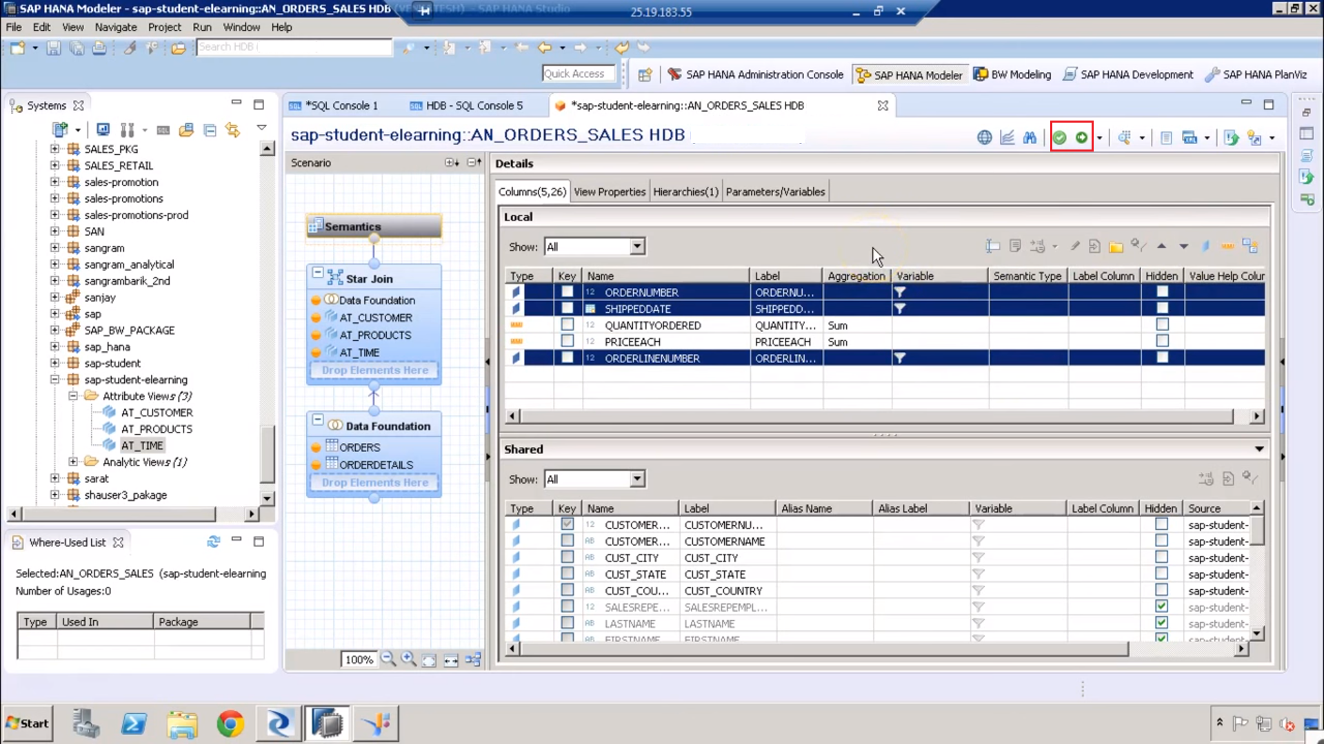
Step 13: After assigning the measures and dimensions, save the Analytic View in SAP HANA Modeler by clicking on the green tick and execute the view by clicking on the green arrow (shown in the red box).

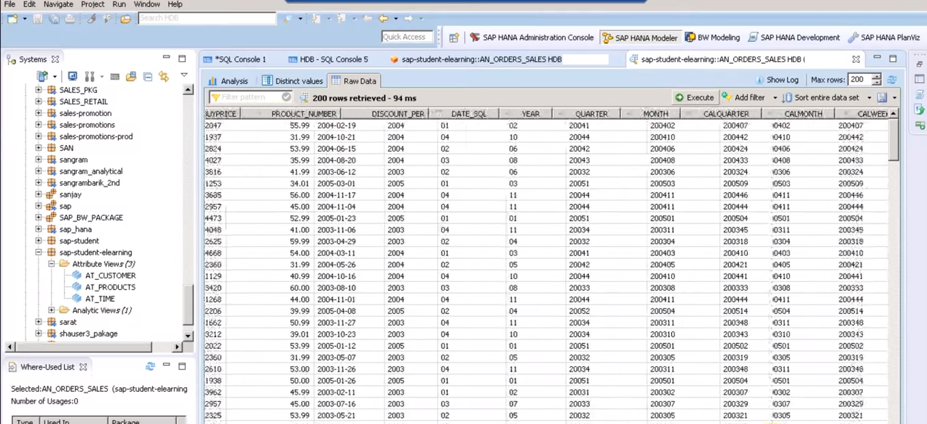
Step 14: After validating and executing it, open the data preview section. There, the raw data from all the tables of the Analytic View in SAP HANA Modeler will get load.

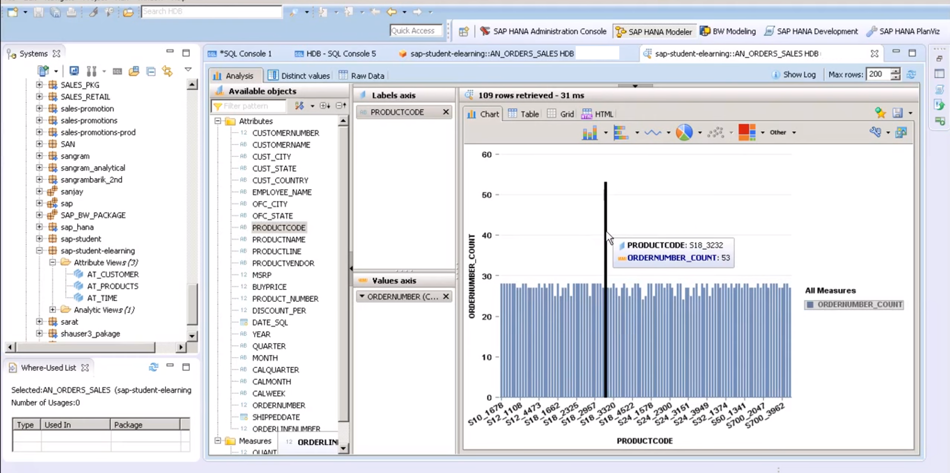
Step 15: From the Analysis section, you can quickly analyze the data by selecting attributes and measures to create different charts and graphs like a bar graph, Mekko chart, pie chart, scatter chart etc.

Summary

We learned about one more Information View in SAP HANA which is the Analytic View. We hope you are understanding the flow of logic as to why these information views are created. In the next lesson, we will learn about a more complex Information View that is Calculation View.

Any doubts or feedbacks regarding the SAP HANA Analytic View article? Simply enter in the comment section.