


Machine Learning courses with 110+ Real-time projects Start Now!!
Hey there, image enthusiasts and fellow curious minds! Have you ever wondered how images undergo those magical transformations you see in computer vision applications? Well, get ready to unlock the secrets of image conversion using the powerful tool known as OpenCV!
As someone who’s always been fascinated by the captivating world of images, I’ve often marvelled at how we can turn a vibrant, colorful snapshot into a monochrome masterpiece or even a stark black-and-white wonderland.
Image conversion lies at the heart of this digital sorcery, and in this article, we’re going to dive into the exciting realm of coloured, grayscale, and binary image processing using OpenCV. Ready? Let’s get this pixel party started!
Why to know Color Space Conversion in OpenCV?
Let’s get to know about the significance of colour space conversion using our beloved image processing tool, OpenCV!
1. Task-specific Advantages: Different color spaces offer specific advantages for various image processing tasks. For instance, HSV is robust to illumination changes, making it suitable for color-based operations.
2. Color Filtering and Isolation: Converting to specific color spaces enables filtering and isolating colors, useful for object detection and segmentation based on color.
3. Efficient Channel Separation: Color space conversion allows easy extraction and manipulation of individual color channels, beneficial for certain image processing operations.
4. Color Correction and Enhancement: Certain color spaces, like LAB, mimic human perception of color, making them useful for color correction and enhancement tasks.
5. Image Compression: Converting to appropriate color spaces can optimize image compression algorithms like JPEG, reducing data redundancy.
6. Visualization and Understanding: Changing color spaces provides alternative visualizations, aiding a better understanding of image content.
7. Compatibility with Algorithms: Some algorithms expect input images in specific color spaces, necessitating conversion for seamless integration.
By leveraging different color representations, OpenCV enhances image processing efficiency and accuracy across a wide range of computer vision applications.
So, What’s cool about grayscale images?
Grayscale images in OpenCV are single-channel images where each pixel’s intensity is represented by a single value, typically ranging from 0 to 255. These images appear in shades of gray, with darker areas having lower intensity values and lighter areas having higher intensity values. Unlike color images that have three color channels (Red, Green, Blue), grayscale images have just one channel, making them more memory-efficient and suitable for certain image processing tasks.
Significance Of Grayscale Images
In OpenCV, grayscale images are commonly used for various purposes :
1. Image Analysis and Feature Extraction:
Grayscale images are often used in tasks like edge detection, contour extraction, and feature extraction. Since these tasks rely on intensity variations rather than color information, grayscale images are sufficient and more straightforward to process.
2. Object Detection and Recognition:
Grayscale images are employed in object detection and recognition tasks, where color information might not be crucial for identifying objects.
3. Image Preprocessing:
Grayscale conversion is an essential preprocessing step before applying various computer vision algorithms. It reduces the computational load and simplifies the analysis process.
4. Medical Imaging:
Grayscale images are commonly used in medical imaging applications, where they provide essential information for diagnoses and medical analyses.
5. Enhancing Image Contrast:
Grayscale images are used in histogram equalization and contrast enhancement techniques to improve image quality and visibility.
6. Machine Learning Applications:
Grayscale images are used as input for certain machine learning models, especially when color information is not necessary for the task at hand.
Grayscale images play a significant role in image processing and computer vision, offering simplicity, efficiency, and suitability for a wide range of applications. They serve as a fundamental representation of visual information, and the study of computer vision and image analysis benefits greatly from their adaptability.
Let’s Convert colored images to grayscale images
Methods of converting Color images to Grayscale using OpenCV:
1. cv2.cvtColor() with cv2.COLOR_BGR2GRAY:
The cv2.cvtColor() method with cv2.COLOR_BGR2GRAY is a commonly used approach to convert a color image to grayscale using OpenCV. This method is straightforward and efficient, making it a popular choice for grayscale conversion.
The cv2.cvtColor() function in OpenCV is specifically designed for color space conversion. Bypassing the cv2.COLOR_BGR2GRAY flag as the conversion parameter, we instruct the function to convert a BGR color image to grayscale.
The cv2.COLOR_BGR2GRAY flag is part of a range of color space conversion codes available in OpenCV, indicating the specific transformation we want to apply. In this case, it maps the color image to a single-channel grayscale image by calculating the weighted sum of the RGB values for each pixel.
Here’s a step-by-step explanation of the process:
1. Load the color image using cv2.imread().
2. Use cv2.cvtColor() with cv2.COLOR_BGR2GRAY to perform the conversion.
We will now use the thresholding method to turn our image black and white. We must use the cv2 module’s threshold function to accomplish this.
In this article, we’ll also use binary thresholding, the most straightforward thresholding method. However, as can be shown above, OpenCV supports additional varieties of thresholding.
As was already said, the binary thresholding procedure relates to the following: each pixel in the image is set to zero if its value is below a specified threshold. If not, a user-defined value is set [3].
3. The result is a grayscale image, with each pixel representing its intensity level, ranging from 0 (black) to 255 (white).
Here’s the code snippet for converting a color image to grayscale using cv2.cvtColor() :
import cv2

# Read the color image
color_image = cv2.imread(cv2.imread(r"C:\Users\satchit\Desktop\DataFlair\Image Conversion using Opencv-colored, grayscale and binary\walking-dog.jpg")

# Convert the color image to grayscale
gray_image = cv2.cvtColor(color_image, cv2.COLOR_BGR2GRAY)

# Display the color image
cv2.imshow("Color Image", color_image)

# Display the grayscale image
cv2.imshow("Grayscale Image", gray_image)

# Wait for a key press and then close all windows
cv2.waitKey(0)
cv2.destroyAllWindows()

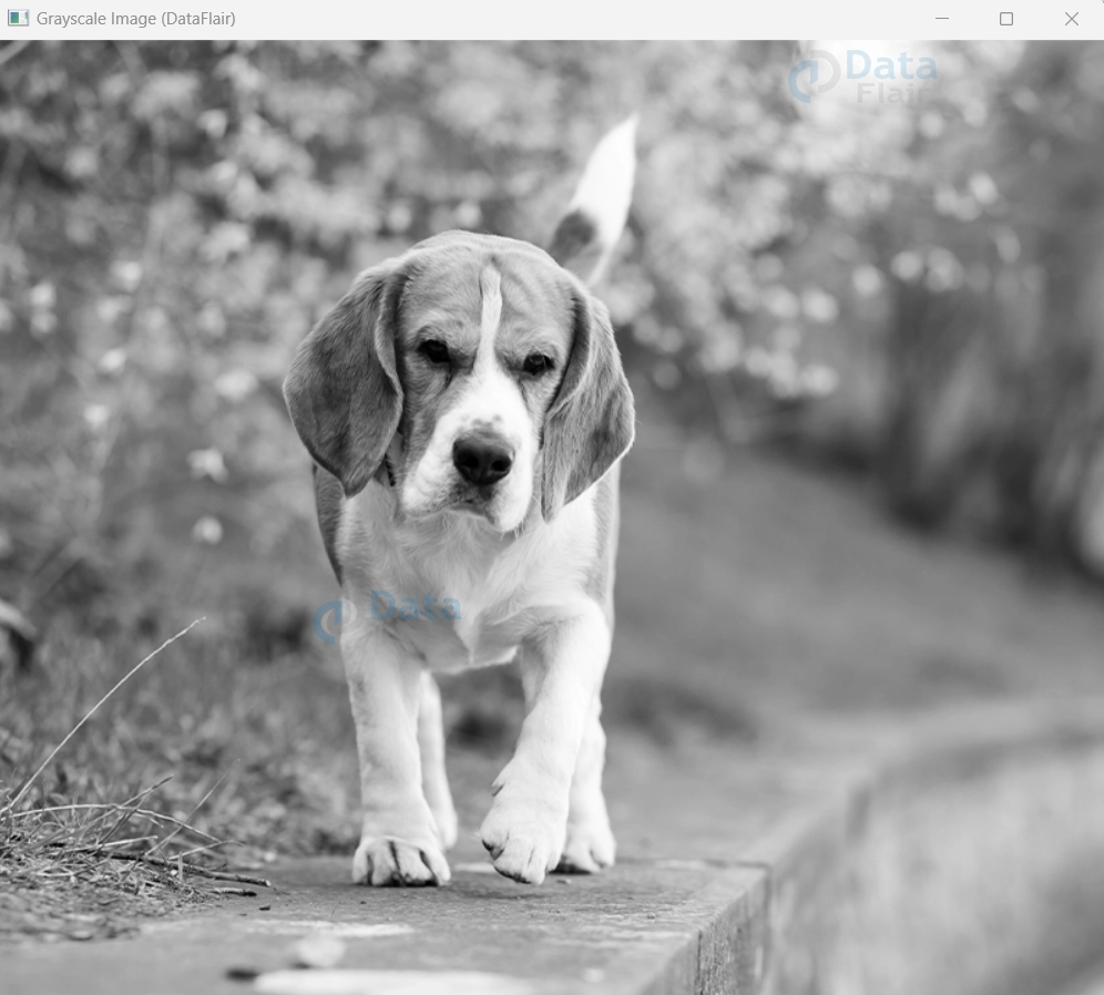
By using cv2.cvtColor() with cv2.COLOR_BGR2GRAY , we can efficiently transform a color image into a grayscale representation, making it easier to perform various image processing tasks that do not require colour information. This method is widely used and considered a standard practice for converting colour images to grayscale using OpenCV.
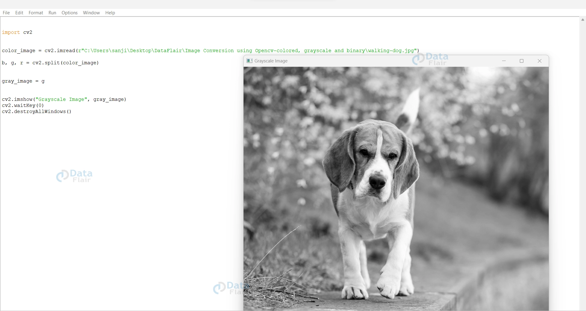
2. cv2.split() and Taking a Single Channel:
The method using cv2.split() and taking a single channel is an alternative approach to converting a colour image to grayscale in OpenCV. While not as common as cv2.cvtColor(), this method allows you to extract a specific colour channel, often the green channel, as the grayscale image.
Let’s elaborate the process in steps:
1. Loading the Color Image: First, we read the color image using the cv2.imread() function and store it in the variable color_image.
import cv2

# Read the color image
color_image = cv2.imread(r"C:\Users\satchit\Desktop\DataFlair\Image Conversion using Opencv-colored, grayscale and binary\walking-dog.jpg")
2. Splitting Color Channels: Next, we use the cv2.split() function to split the color channels of the image into individual channels. The function returns a tuple containing separate images for each color channel (blue, green, and red).
# Split the color channels
b, g, r = cv2.split(color_image)
3. Choosing the Green Channel as Grayscale Image: After splitting the channels, we select one of them to be the grayscale image. The green channel (`g`) is commonly chosen as it provides a reasonable approximation of the overall intensity in the image.
# Take the green channel as the grayscale image
gray_image = g
4. Displaying the Grayscale Image: Finally, we display the grayscale image using the cv2.imshow() function. It will open a window showing the grayscale representation of the original color image.
# Display the grayscale image
cv2.imshow("Grayscale Image", gray_image)
cv2.waitKey(0)
cv2.destroyAllWindows()
- The above code will open two windows: one displaying the original color image and another showing the grayscale image extracted from the green channel.
- By using the green channel as the grayscale image, we leverage the fact that the human eye is most sensitive to green, making it a suitable representation of the overall intensity of the image.
- While this approach provides an alternative way to convert to grayscale, it is less commonly used than the cv2.cvtColor() method, which is simpler and more straightforward.
- However, cv2.split() can be useful when you want to perform specific manipulations on individual colour channels or when you have a specific reason to use a particular colour channel as the grayscale image.
Here’s the full code:
import cv2

# Read the color image
color_image = cv2.imread(r"C:\Users\satchit\Desktop\DataFlair\Image Conversion using Opencv-colored, grayscale and binary\walking-dog.jpg")

# Split the color channels
b, g, r = cv2.split(color_image)

# Take the green channel as the grayscale image
gray_image = g

# Display the grayscale image
cv2.imshow("Grayscale Image", gray_image)
cv2.waitKey(0)
cv2.destroyAllWindows()
3. The Weighted Averaging Method:
The Weighted Averaging Method is a manual approach to converting a colour image to grayscale by calculating the grayscale intensity of each pixel through a weighted average of its RGB (Red, Green, Blue) color values. This method allows fine-tuning the conversion based on specific requirements.
Check out these steps:
1. Load the color image using `cv2.imread()` function.
2. Iterate through each pixel of the color image.
3. For each pixel, calculate the grayscale intensity using the weighted average of the RGB values.
4. Set the grayscale intensity value for that pixel in the grayscale image.
5. Display the grayscale image using cv2.imshow() function.
Here’s the code implementing the Weighted Averaging Method:
import cv2

# Read the color image
color_image = cv2.imread(r"C:\Users\satchit\Desktop\DataFlair\Image Conversion using Opencv-colored, grayscale and binary\walking-dog.jpg")

# Create an empty grayscale image with the same dimensions as the color image
gray_image = np.zeros_like(color_image[:, :, 0])

# Calculate the weighted average of RGB values to get grayscale intensity
height, width = color_image.shape[:2]
for y in range(height):
    for x in range(width):
        b, g, r = color_image[y, x]
        gray_intensity = 0.299 * r + 0.587 * g + 0.114 * b
        gray_image[y, x] = gray_intensity

# Display the grayscale image
cv2.imshow("Grayscale Image", gray_image)
cv2.waitKey(0)
cv2.destroyAllWindows()
In this code, we manually calculate the grayscale intensity for each pixel using the formula:
Gray Intensity = 0.299 * Red + 0.587 * Green + 0.114 * Blue
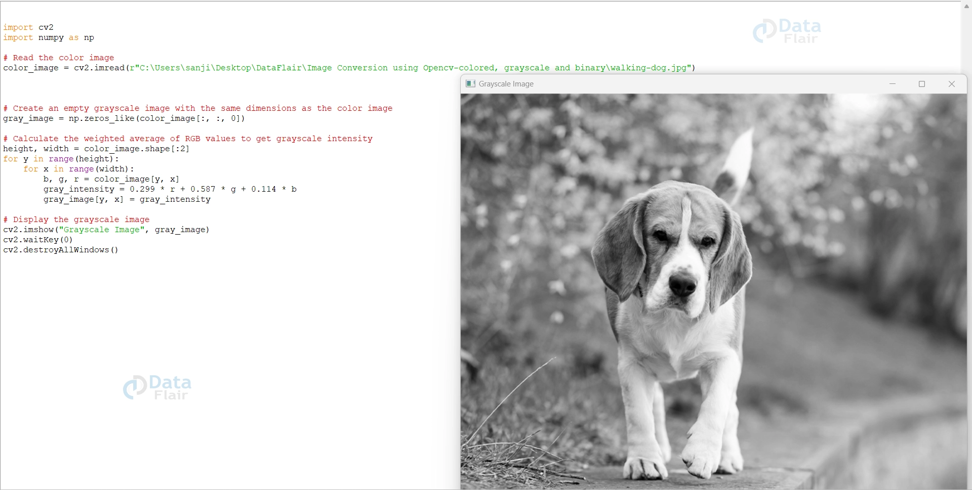
The weights (0.299, 0.587, and 0.114) represent the sensitivity of the human eye to the red, green, and blue colors, respectively. The calculated grayscale intensity is assigned to the corresponding pixel in the grayscale image.
Please note that the first method uses cv2.cvtColor() with the flag cv2.COLOR_BGR2GRAY is simpler and more commonly used for converting color images to grayscale. However, the Weighted Averaging Method provides more control over the conversion process and can be useful in specific situations where fine-tuning is required.
Converting Images to Binary images using OpenCV
To convert an image to binary using OpenCV, you can use the cv2.threshold() function. This function applies a threshold to a grayscale image, converting it to a binary image.
The cv2.threshold() function in OpenCV is used to apply a threshold to a grayscale image, effectively converting it into a binary image. Thresholding is a simple image segmentation technique that separates pixels into two categories based on their intensity values relative to a specified threshold.
Here’s the syntax of the cv2.threshold() function:
retval, threshold_image = cv2.threshold(src, thresh, maxval, type)
- src: This is the input grayscale image (single-channel image) on which the thresholding operation will be applied.
- Thresh: The threshold value. Pixels with intensity values below this threshold will be set to `0`, and pixels with intensity values above or equal to this threshold will be set to `maximal`.
- maxval: The maximum value to use when a pixel’s intensity value is above or equal to the threshold. Typically, this is set to `255` for binary thresholding to create a binary image with black (0) and white (255) pixels.
- Type : The thresholding type. It specifies how the thresholding operation will be applied. Some commonly used types are:
- cv2.THRESH_BINARY: Binary thresholding. Pixels below the threshold are set to 0, and pixels above or equal to the threshold are set to `maxval`.
- cv2.THRESH_BINARY_INV: Inverse binary thresholding. Pixels below the threshold are set to `maxval`, and pixels above or equal to the threshold are set to 0.
- cv2.THRESH_TRUNC: Thresholding with truncation. Pixels above the threshold are set to the threshold value, and pixels below the threshold remain unchanged.
- cv2.THRESH_TOZERO: Thresholding to zero. Pixels below the threshold are set to 0, and pixels above or equal to the threshold remain unchanged.
- cv2.THRESH_TOZERO_INV: Inverse thresholding to zero. Pixels below the threshold are set to their original value, and pixels above or equal to the threshold are set to 0.
The cv2.threshold() function returns two values:
- Retval: The threshold value that was used (not often used, usually denoted by an underscore `_` as it is not needed).
- Threshold_image: The output binary image resulting from the thresholding operation.
The cv2.threshold() function is a fundamental tool for image segmentation and is commonly used in various image processing applications.
Here’s a step-by-step code to achieve binary image processing :
import cv2

# Read the color image (if needed)
color_image = cv2.imread(r"C:\Users\satchit\Desktop\DataFlair\Image Conversion using Opencv-colored, grayscale and binary\walking-dog.jpg")

# Convert the color image to grayscale
gray_image = cv2.cvtColor(color_image, cv2.COLOR_BGR2GRAY)

# Apply thresholding to create a binary image
_, binary_image = cv2.threshold(gray_image, 127, 255, cv2.THRESH_BINARY)

# Display the binary image
cv2.imshow("Binary Image", binary_image)
cv2.waitKey(0)
cv2.destroyAllWindows()
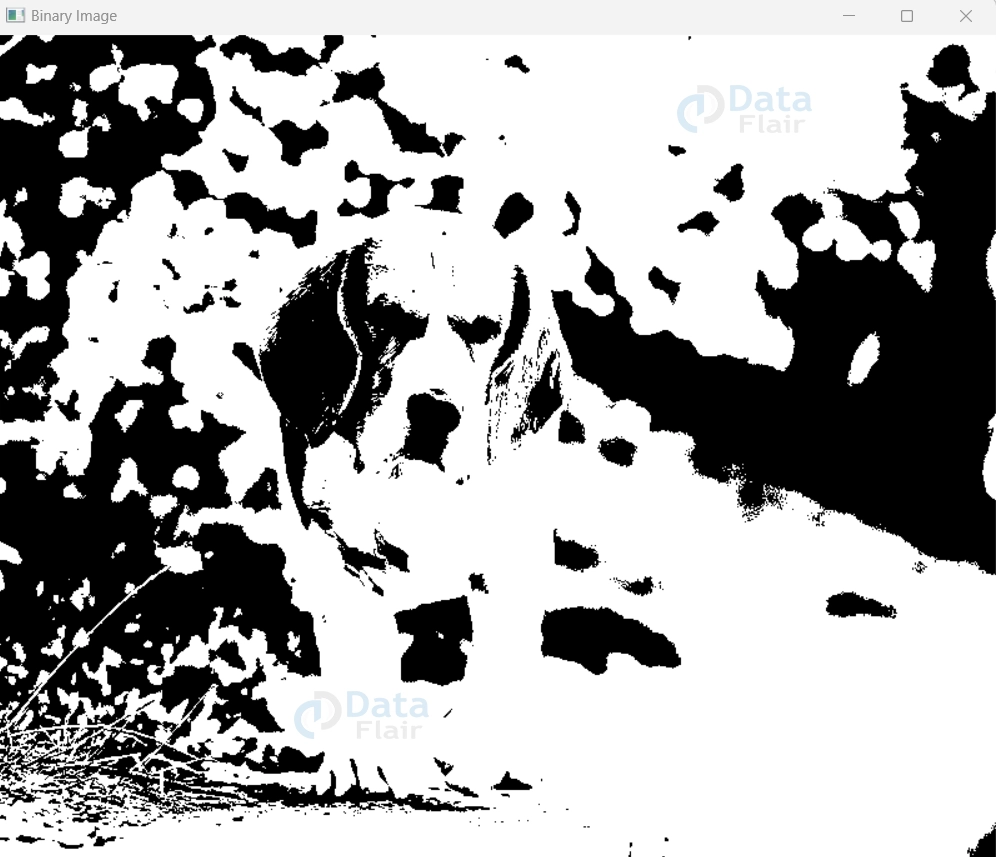
In this code, we first read the color image using cv2.imread() (if your image is not already in grayscale). Then, we convert the color image to grayscale using cv2.cvtColor() with the flag cv2.COLOR_BGR2GRAY.
Next, we apply thresholding to the grayscale image using cv2.threshold(). The function takes several arguments:
- The first argument is the grayscale image.
- The second argument is the threshold value. Pixels with values below this threshold will become 0 (black), and those above or equal to it will become 255 (white).
- The third argument is the maximum value to be assigned to pixels above the threshold. Here, we set it to 255 to get a binary image with black and white pixels.
- The fourth argument is the thresholding method. We use cv2.THRESH_BINARY, which is the basic binary thresholding method.
The cv2.threshold() function returns two values: the threshold value used (here, it is denoted by `_`, as it is not needed) and the binary image.
Finally, we display the binary image using cv2.imshow() and then wait for a key press before closing all the windows using cv2.waitKey(0) and cv2.destroyAllWindows().
The resulting binary image will contain only black and white pixels, with black representing values below the threshold and white representing values above or equal to the threshold.
Summary
In this article, we explored the process of image conversion using OpenCV, a powerful library for computer vision and image processing. The primary focus was on transforming color images into grayscale and binary representations, each serving different purposes and applications. The straightforward approach using cv2.cvtColor() with cv2.COLOR_BGR2GRAY was presented, followed by a more manual method of using cv2.split().
We introduced the Weighted Averaging Method, a unique way to convert color images to grayscale by calculating the intensity of each pixel using weighted averages of RGB values. Various thresholding techniques, including binary, binary inverse, truncation, to zero, and to zero inverse, were briefly discussed.