Principal Components and Factor Analysis in R – Functions & Methods

With this tutorial, learn about the concept of principal components, reasons to use it and different functions and methods of principal component analysis in R programming. Also, understand the complete technique of factor analysis in R.

Introduction to Principal Components and Factor Analysis in R

Thus, it is always performed on a symmetric correlation or covariance matrix. Hence, it means the matrix should be numeric.

Wait! Before proceeding ahead, make sure to complete the R Matrix Function Tutorial

What are Principal Components in R?

It is a normalized linear combination of the original predictors in a data set. We can write the principal component in the following way:

Z¹ = Φ¹¹X¹ + Φ²¹X² + Φ³¹X³ + …. +Φp¹Xp

where,

Z¹ is the first principal component.

Φp¹ is the loading vector comprising of loadings (Φ¹, Φ²..) of a first principal component.

Also, the loadings are constrained to a sum of square equal to 1. This is because the large size of loadings may lead to large variance. The direction of the principal component (Z¹) which has the highest variation of data is also defined. Moreover, it results in a line in p dimensional space which is closest to the n observations. We can measure closeness using average squared Euclidean distance.

X¹..Xp is normalized predictors. The means of normalized predictors are equal to 0 and have a standard deviation of 1.

Why use Principal Components Analysis?

The main aim of principal components analysis in R is to report hidden structure in a data set. In doing so, we may be able to do the following things:

• Basically, it is prior to identifying how different variables work together to create the dynamics of the system.
• Reduce the dimensionality of the data.
• Decreases redundancy in the data.
• Filter some of the noise in the data.
• Compress the data.
• Prepare the data for further analysis using other techniques.

Functions to Perform Principal Analysis in R

1. prcomp() (stats)
2. princomp() (stats)
3. PCA() (FactoMineR)
4. dudi.pca() (ade4)
5. acp() (amap)

Implementing Principal Components Analysis in R

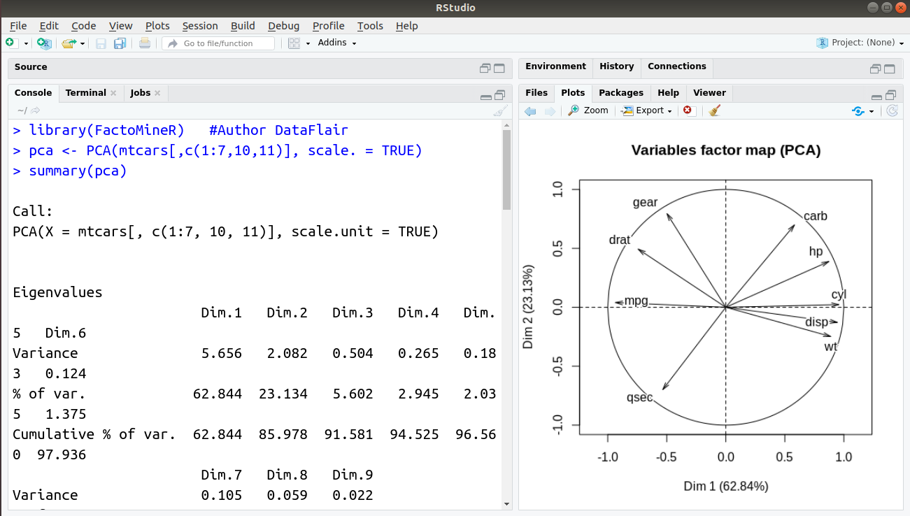
We will now proceed towards implementing our own Principal Components Analysis (PCA) in R. For carrying out this operation, we will utilise the pca() function that is provided to us by the FactoMineR library. We will make use of the mtcars dataset which is provided to us by R. In this dataset, there are total 11 features out of which we require 9 features as two of them are categorical in nature. We will then have a look at our PCA objects with the help of summary() function.

> library(FactoMineR)   #Author DataFlair
> pca <- PCA(mtcars[,c(1:7,10,11)], scale. = TRUE)
> summary(pca)

Output:

In order to display the matrix with its constituent eigenvalues, we will write the following code:

> pca$eig #Author DataFlair

Output:

Furthermore, for finding correlations between variables and their correlations, we write the following line of code:

> pca$var$coord #DataFlair

Output:

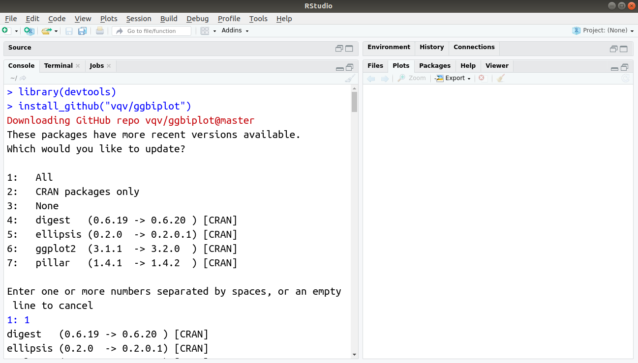
While the default graph provided to us by the PCA() function is good, we can choose to create a better visualisation of our data using the ggbiplot library. You can install this package as follows:

> library(devtools)
> install_github("vqv/ggbiplot")

Output:

Finally, we import this package and plot our PCA graph:

> library(ggbiplot)  #AuthorDataFlair
> ggbiplot(pca)

Output:

Grab a complete tutorial on R Recursive Function

Methods for Principal Component Analysis in R

There are two methods for R principal component analysis:

1. Spectral Decomposition

It examines the covariances/correlations between variables.

2. Singular Value Decomposition

It examines the covariances/correlations between individuals. Function princomp() is used here for carrying out a spectral approach.  And, we can also use the functions prcomp() and PCA() in the singular value decomposition.

prcomp() and princomp() functions

The simplified format of these two functions are :

• prcomp(x, scale = FALSE)
• princomp(x, cor = FALSE, scores = TRUE)

Arguments for prcomp()

• x: A numeric matrix or data frame.
  
• scale: It is a logical value. It indicates whether the variables should be scaled to have unit variance and will take place before the analysis takes place.

Arguments for princomp()

• x: A numeric matrix or data frame.
  
• cor: A logical value. If TRUE, then data will be centred and also scaled before the analysis.
  
• scores: A logical value. If TRUE, then coordinates on each principal component are calculated.

Factor Analysis in R

Exploratory Factor Analysis or simply Factor Analysis is a technique used for the identification of the latent relational structure. Using this technique, the variance of a large number can be explained with the help of fewer variables.

Let us understand factor analysis through the following example:

Assume an instance of a demographics based survey. Suppose that there is a survey about the number of dropouts in academic institutions. It is observed that the number of dropouts is much greater at higher levels of institutions. That is, the number of high school dropouts is much higher than in junior school. Similarly, the number of dropouts in college is much higher than in high school. In this case, the driving factor behind the number of dropouts is the increase in academic difficulty. But besides this, there can be many other factors like financial background, localities with higher pupil-teacher ratio and even gender in the most remote parts. Since there are multiple factors that contribute towards the dropout rate, we have to define variables in a structured and a defined manner. The main principle of factor analysis is the categorization of weights based on the influence that the category has. 

With factor analysis, we are able to assess the variables that are hidden from plain observation but are reflected in the variables of the data. We perform the transformation on our dataset to an equal number of variables such that each variable is a combination of the current ones. This is performed without any removal or addition of new information. Therefore, the transformation of these variables in the direction of eigenvalues will help us to determine influential factors. Eigenvalue having a value more than 1 will have greater variance than the original one. These factors are then arranged in a decreasing format based on their variances. Therefore, the first factor will have a higher variance than the second one and so on. Weights that contribute towards the variance are known as ‘factor loadings’.

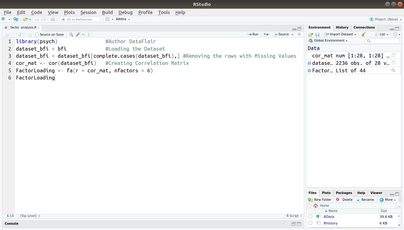
Now, let us take a practical example of factor analysis in R. We will use the BFI dataset that comprises of personality items. There are about 2800 data points with five main factors – A (Agreeableness), C (Conscientiousness), E (Extraversion), N (Neuroticism), O (Openness). We will implement factor analysis to assess the association of the variables with each factor. 

library(psych)                #Author DataFlair
dataset_bfi = bfi             #Loading the Dataset
dataset_bfi = dataset_bfi[complete.cases(dataset_bfi),] #Removing the rows with Missing Values
cor_mat <- cor(dataset_bfi)   #Creating Correlation Matrix 
FactorLoading <- fa(r = cor_mat, nfactors = 6)
FactorLoading

Code Display:

Output:

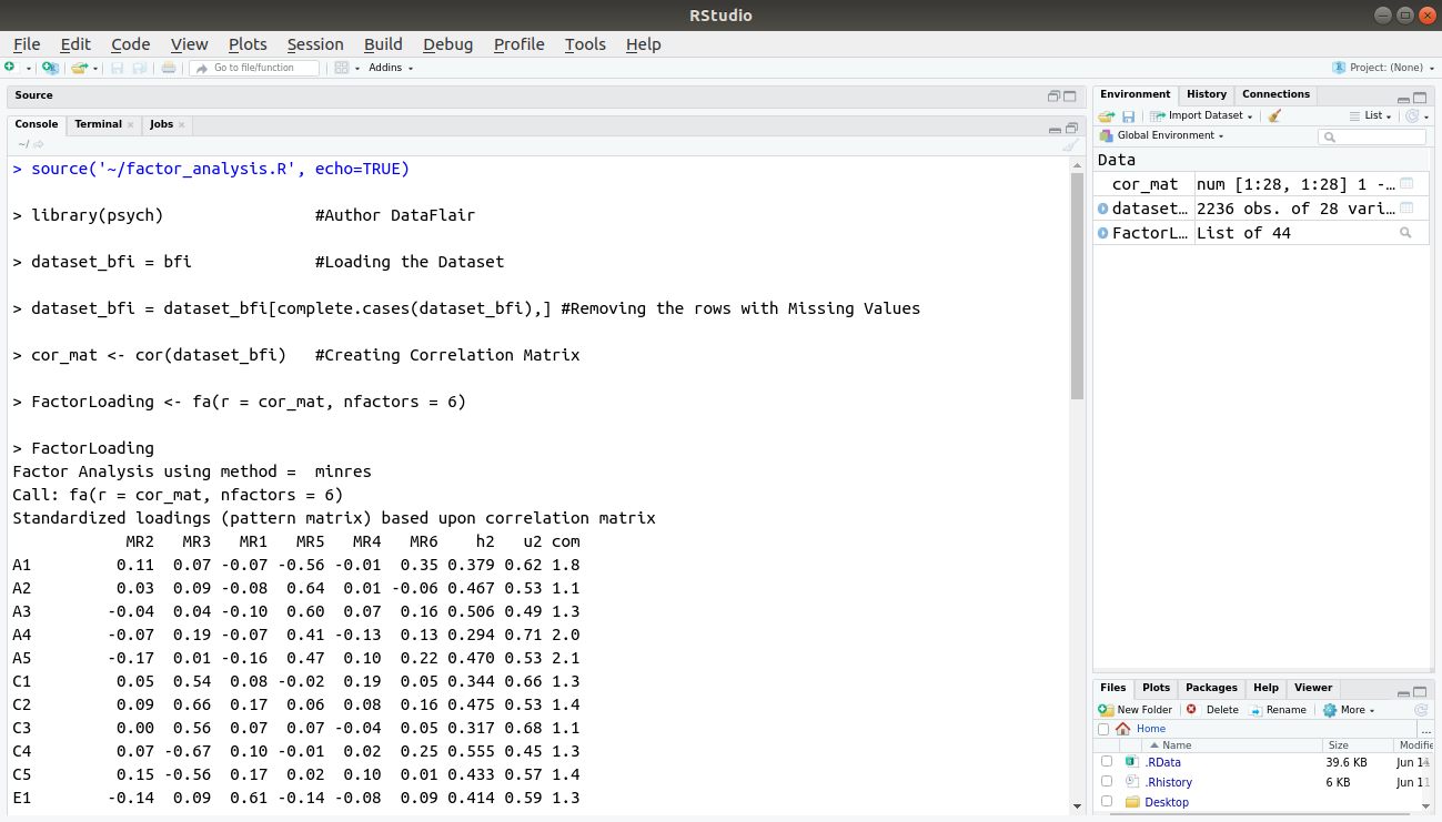
From the above output, we observe that the first factor N has the highest variance among all the variables. We infer that most members have neuroticism in our data.

Summary

We have studied the principal component and factor analysis in R. Along with this, we have also discussed its usage, functions, components.

Now, it’s time for learning the Major Functions to Organise the data with R Data Reshaping Tutorial

Feel free to share your thoughts in the comment section below. Hope you enjoyed learning!!