Bayes’ Theorem – The Forecasting Pillar of Data Science
Free Machine Learning courses with 130+ real-time projects Start Now!!
Are you planning to become a data scientist? If yes, you must read this extensive article on Bayes’ Theorem for Data Science.
No data scientist can work without a complete understanding of conditional probability and Bayesian inference. So, today, we will discuss the same with the help of examples and applications. More importantly, we will discuss how Data Scientist use Bayes’ Theorem.
Bayes’ Theorem is the most important concept in Data Science. It is most widely used in Machine Learning as a classifier that makes use of Naive Bayes’ Classifier. It has also emerged as an advanced algorithm for the development of Bayesian Neural Networks.
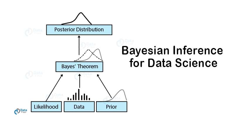
The applications of Bayes’ Theorem are everywhere in the field of Data Science. Let us first have an overview of what exactly Bayes’ Theorem is.
What is Bayes’ Theorem?
Bayes’ Theorem is the basic foundation of probability. It is the determination of the conditional probability of an event. This conditional probability is known as a hypothesis. This hypothesis is calculated through previous evidence or knowledge.
This conditional probability is the probability of the occurrence of an event, given that some other event has already happened.
The formula of Bayes’ Theorem involves the posterior probability P(H | E) as the product of the probability of hypothesis P(E | H), multiplied by the probability of the hypothesis P(H) and divided by the probability of the evidence P(E).
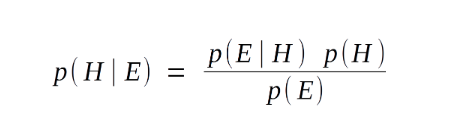
Let us now understand each term of the Bayes’ Theorem formula in detail –
- P(H | E) – This is referred to as the posterior probability. Posteriori basically means deriving theory out of given evidence. It denotes the conditional probability of H (hypothesis), given the evidence E.
- P(E | H) – This component of our Bayes’ Theorem denotes the likelihood. It is the conditional probability of the occurrence of the evidence, given the hypothesis. It calculates the probability of the evidence, considering that the assumed hypothesis holds true.
- P(H) – This is referred to as the prior probability. It denotes the original probability of the hypothesis H being true before the implementation of Bayes’ Theorem. That is, this probability is without the involvement of the data or the evidence.
- P(E) – This is the probability of the occurrence of evidence regardless of the hypothesis.
You must take a look at – K-means Clustering Tutorial
Bayes’ Theorem Example
Let us assume a simple example to understand Bayes’ Theorem. Suppose the weather of the day is cloudy. Now, you need to know whether it would rain today, given the cloudiness of the day. Therefore, you are supposed to calculate the probability of rainfall, given the evidence of cloudiness.
That is, P(Rain | Clouds), where finding whether it would rain today is the Hypothesis (H) and Cloudiness is the Evidence (E). This is the posterior probability part of our equation.
Now, suppose we know that 60% of the time, rainfall is caused by cloudy weather. Therefore, we have the probability of it being cloudy, given the rain, that is P(clouds | rain) = P(E | H).
This is the backward probability where, E is the evidence of observing clouds given the probability of the rainfall, which is originally our hypothesis. Now, out of all the days, 75% of the days in a month are cloudy. This is the probability of cloudiness or P(clouds).
Also, since this is a rainy month of the year, it rains usually for 15 days out of 30 days. That is, the probability of hypothesis of rainfall or P(H) is P(Rain) = 15/30 = 0.5 or 50%. Now, let us calculate the probability of it raining, given the cloudy weather.
P(Rain | Cloud) = (P(Cloud | Rain) * P(Rain)) / (P(Cloud))
= (0.6 * 0.5) / (0.75)
= 0.4
Therefore, we find out that there is a 40% chance of rainfall, given the cloudy weather.
After understanding Bayes’ Theorem, let us understand the Naive Bayes’ Theorem. The Naive Bayes’ theorem is an implementation of the standard theorem in the context of machine learning.
Do you know the importance of R for Data Scientists?
Naive Bayes Theorem
Naive Bayes is a powerful supervised learning algorithm that is used for classification. The Naive Bayes classifier is an extension of the above discussed standard Bayes Theorem. In a Naive Bayes, we calculate the probability contributed by every factor.
Most we use it in textual classification operations like spam filtering. Let us understand how Naive Bayes calculates the probability contributed by all the factors.
Suppose that, as a data scientist, you are tasked with developing a spam filter. You are provided with a list of spam keywords such as
- Free
- Discount
- Full Refund
- Urgent
- Weight Loss
However, the company you are working with is a product finance company. Therefore, some of the vocabulary occurring in the spam mails is used in the mails of your company. Some of these words are –
- Important
- Free
- Urgent
- Stocks
- Customers
You also have the probability of word usages in spam messages and company emails.
| Spam Email | Company Email |
| Free (0.3) | Important (0.5) |
| Discount (0.15) | Free (0.25) |
| Full Refund (0.1) | Urgent (0.1) |
| Urgent (0.2) | Stocks (0.5) |
| Weight Loss (0.25) | Customers (0.1) |
Suppose you obtain have a message “Free trials for weight loss program. Become members at a discount.” Is this message spam or a company email? Calculating the probability of the components occurring in the sentence – Free (0.4) + Weight Loss (0.25) + Discount (0.15) = 0.8 or 80%
Whereas, calculating the probability of it being an email from your company = Free (0.25) = 0.25 or 25%.
Therefore, the probability of the mail being spam is much higher than a company email.
A Naive Bayes Classifier selects the outcome of the highest probability, which in the above case was the feature of spam.
The Naive Bayes is referred to as ‘naive’ because it assumes the features to be independent of each other. The features in our example were the input words that are present in the sentence.
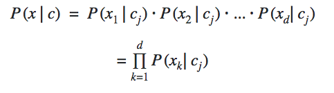
The conditional independence among all the features gives us the formula above. The frequency of the occurrence of features from x1 to xdis calculated based on their relation to the class cj.
Along with the prior probability and the probability of the occurrence of an event, we calculate the posterior probability through which we are able to find the probability of the object belonging to a particular class.
Along with this Bayes’ Theorem, Data Scientists use various different tools. You must check the different tools used by a Data Scientist.
Using Naive Bayes as a Classifier
In this section, we will implement the Naive Bayes Classifier over a dataset. The dataset used in this example is the Pima Indian Dataset which is an open dataset available at the UCI Library.
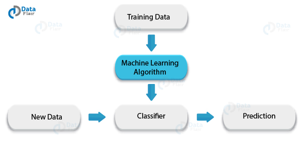
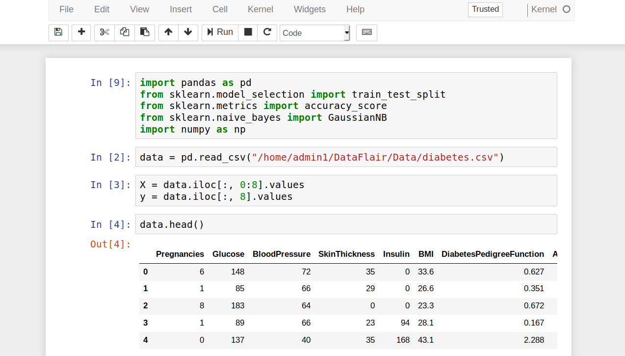
- In the first step, we import all the libraries that will allow us to implement our Naive Bayes Classifier and help us in wrangling the data.
import pandas as pd
from sklearn.model_selection import train_test_split
from sklearn.metrics import accuracy_score
from sklearn.naive_bayes import GaussianNB
- We then read the csv file through an online URL using read_csv function provided by the Pandas library.
data = pd.read_csv("/home/admin1/DataFlair/Data/diabetes.csv")- Then, we proceed to divide our data into dependent variable (Y) and independent variables(X) as follows –
X = data.iloc[:, 0:8].values
y = data.iloc[:, 8].values
- Using the head() function provided by the Pandas library, we look at the first five rows of our dataset.
data.head()
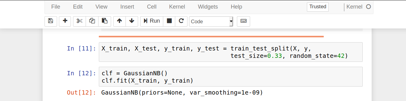
- We then proceed to split our dataset into training and validation sets. We will train our Naive Bayes Classifier on the training set and generate predictions from the test set. In order to do so, we will use the train_test_split() function provided by the sklearn library.
X_train, X_test, y_train, y_test = train_test_split(X, y, test_size=0.33, random_state=42)
- In this step, we apply the Naive Bayes Classifier and more specifically, the Gaussian Naive Bayes Classifier. It is an extension of the existing Naive Bayes Classifier that assumes the likelihood of the features to be Gaussian or normally distributed.
clf = GaussianNB()
clf.fit(X_train, y_train)
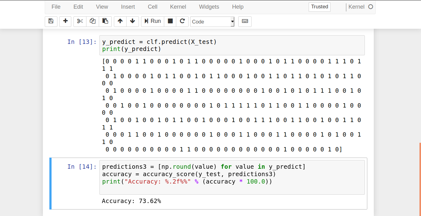
- In the next step, we generate predictions from our given test sample.
y_predict = clf.predict(X_test)
print(y_predict)
- Then, we measure the accuracy of our classifier. That is, we test to see how many values were predicted correctly.
predictions3 = [np.round(value) for value in y_predict]
accuracy = accuracy_score(y_test, predictions3)
print("Accuracy: %.2f%%" % (accuracy * 100.0))
Therefore, our Naive Bayes Classifier predicted 72.44% of the test-cases successfully.
Recommended Reading – Top Data Science Use Cases
Applications of Bayes’ Theorem
1. Spam Filtering
The first and foremost application of Naive Bayes is its ability to classify texts and in particular, spam emails from non-spam ones.
It is one of the oldest spam filtering methodology, with the Naive Bayes spam filtering dating back to 1998. Naive Bayes takes two classes – Spam and Ham and classifies data accordingly.
2. Sentiment Analysis
It is a part of natural language processing that analyzes if the data is positive, negative or neutral. Another terminology for Sentiment Analysis is opinion mining. Using Naive Bayes, we can classify if the text is positive or negative or determine what class the sentiment of the person belongs to.
3. Recommendation Systems
Using Naive Bayes we can build recommendation systems. A recommendation system measures the likelihood of the person watching a film or not, given the past watches. It is also used in conjunction with collaborative filtering to filter information for the users.
4. Bayesian Neural Networks
Recently, Bayes’ Theorem has been extended into Deep Learning where it is used to design powerful Bayesian Networks. It is then used in complex machine learning tasks like stock forecasting, facial recognition etc. It is a currently trending topic and has revolutionized the field of deep learning.
Summary
In the end, we conclude that the use of Bayes’ Theorem is for finding the conditional probability of an event. It has several extensions that are used in Data Science such as Naive Bayes, Gaussian Naive Bayes’, Gaussian Neural Networks etc.
Hope now you are clear with the concept of Bayes’ Theorem for Data Science. And if any doubts, you can freely ask through comments.
You must read another interesting article – How to get your first job in Data Science?
Did you like our efforts? If Yes, please give DataFlair 5 Stars on Google


Free (0.4) + Weight Loss (0.25) + Discount (0.15) = 0.8 or 80%
Shouldn’t it be Free(0.3)?
Your formula says we should multiply the probability of occurring words, not adding them. I think your example (calculations) are wrong about Naive Bayes Theorem