Descriptive Statistics in R – Complete Guide for aspiring Data Scientists!
FREE Online Courses: Elevate Your Skills, Zero Cost Attached - Enroll Now!
This article will provide you with a comprehensive explanation of the descriptive statistics in R programming also known as summary statistics. We will learn these R commands along with their use and implementation with the help of examples.
- summary
- name
- apply
- simple cumulative
- complex cumulative
What is Summary Statistics/Descriptive Statistics?
All the data which is gathered for any analysis is useful when it is properly represented so that it is easily understandable by everyone and helps in proper decision making. After we carry out the data analysis, we delineate its summary so as to understand it in a much better way. This is known as summarizing the data.
We can summarize the data in several ways either by text manner or by pictorial representation.
We can summarize our data in R as follows:
- Descriptive/Summary Statistics – With the help of descriptive statistics, we can represent the information about our datasets. They also form the platform for carrying out complex computations as well as analysis. Therefore, even though they are developed with simple methods, they play a crucial role in the process of analysis.
- Tabulation – Representing the data analyzed in tabular form for easy understanding.
- Graphical – It is a way to represent data graphically.
I hope you have completed the tutorial on Data Manipulation in R before proceeding ahead.
Summary Commands in R
Whenever you start working on any data set, you need to know the overview of what you are dealing with. There are a few ways of doing this:
As we have seen in the earlier session that ls() command is used to know the list of named objects that you have. So you can start by using ls command for this purpose.
Once you know the objects that are available, you can then type the name of the object to view its content. However, if the object contains a lot of data, the display may be quite large and you may want a more concise method to examine objects.
You could use the str() command which shows you something about the structure of data rather than giving the statistical summary. It will inform you about the number of rows and columns in the data and values in the columns with their respective heads. The str() command is designed to help you examine the structure of a data object rather than providing a statistical summary.
The summary() command will provide you with a statistical summary of your data.
The output of summary command depends on the object you are looking at. It gives the output as the largest value in data, the least value or mean and median and another similar type of information.
For example, if you have below data:
S.No. Item Quantity
1 Pen 5
2 Pencil 10
3 Rubber 12
#Author DataFlair
data <- read.table(header=TRUE, text='
S.No. Item Quantity
1 Pen 5
2 Pencil 10
3 Rubber 12
')
str(data)    #description of the output
summary(data)  #statistical summary
Output:
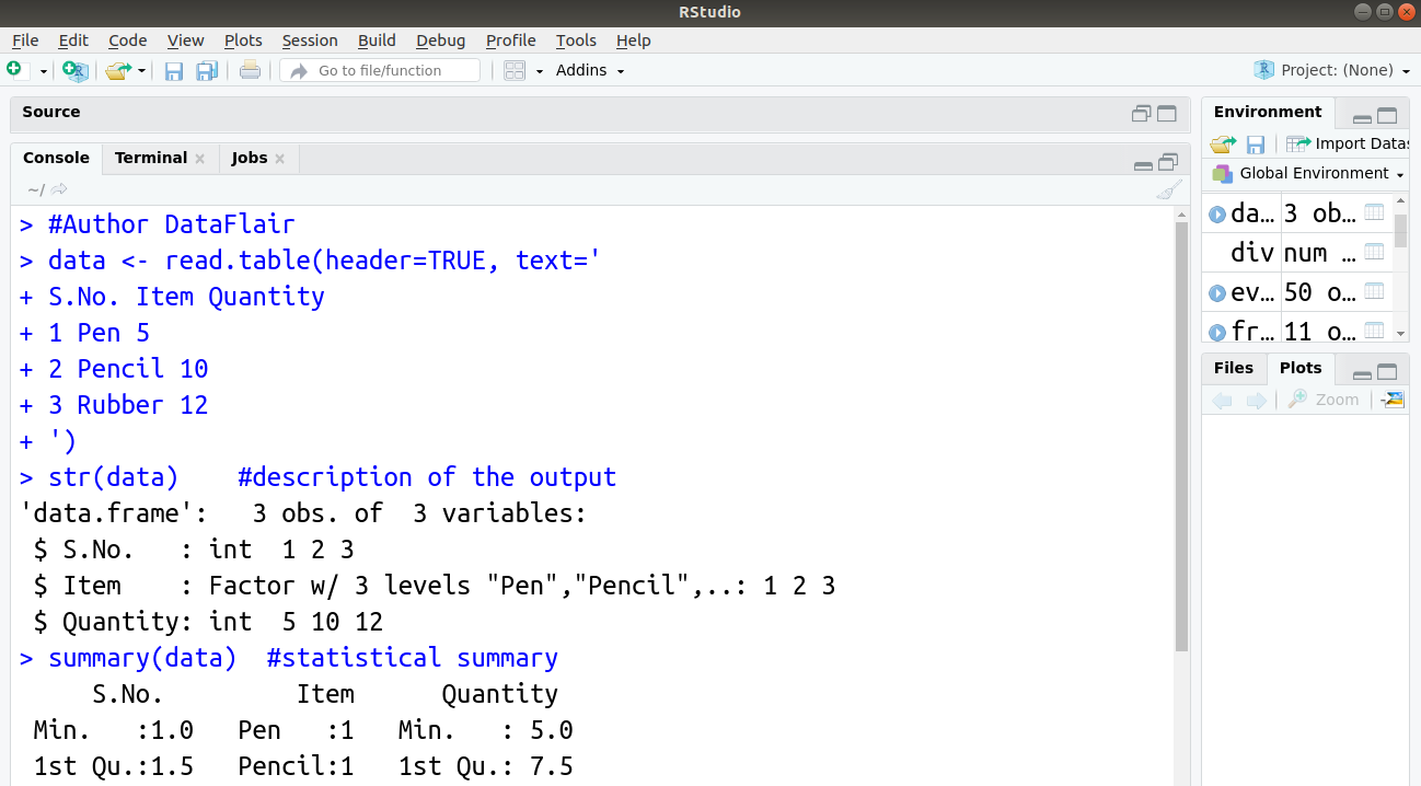
The summary command is, therefore, more useful as we can see minimum, maximum, mean, etc values. The summary() command works for both matrix and data frame objects by summarizing the columns rather than the rows.
Don’t miss the concept of Object Oriented Programming in R
Name Commands in R
Name command and its variants are used to find or add names to rows and columns of data structures.
Below specified are few of the commands and their explanation:
- names() – It works on matrix or data frame objects.
- rownames() – It works on matrix or data frame objects and is used to give names to rows.
- colnames() – It works on matrix or data frame objects and is used to give names to columns.
- dimnames() – Gets row and column names for matrix or data frame objects, that is, it is used to see dimensions of the data frame.
rownames and row.names return the same values for the data frame and matrices; the only difference is that where there aren’t any names present, rownames will print “NULL” (as does colnames), but row.names return it invisibly.
Descriptive statistics is used to analyze data in various types of industries, such as education, information technology, entertainment, retail, agriculture, transport, sales and marketing, psychology, demography, and advertising. In a broader sense, it is used as a tool to interpret and analyze data. For example – With the help of descriptive statistics, a production engineer can uncover the truth behind the breakdown of motors and a manager can supervise the quality of the production process.
Summarizing Samples in R Programming Language
When repeated measurements are there, we generally want to summarize data by showing measures like average. R provides a variety of commands that operate on samples. These samples of data might be individual vectors, or they may be columns in a data frame or part of a matrix or list.
Let’s suppose a survey is conducted to find the average weight of people living in a country. As it is not possible to weigh every person of the country, a sample data of a few thousand individuals is collected. The average weight of the people in the sample would be very near to the average weight of the entire population of that country.
A variety of simple summary statistics can be applied to a vector of numbers. Two kinds of summary commands used are:
- Commands for Single Value Results – Produce single value as a result.
- Commands for Multiple Value Result – Produce multiple results as an output.
The next essential concept in R descriptive statistics is the summary commands with single value results.
Take a deep insight into R Vector Functions
Summary Commands with Single Value Results in R
There are many such commands that produce a single value as output. Let us see a few of them:
- max(x, na.rm = FALSE) – It shows the maximum value. By default, NA values are not removed. NA is considered the largest unless na.rm=true is used.
- min(x, na.rm = FALSE) – Shows minimum value in a vector. If there are na values, NA is returned unless na.rm=true is used.
- length(x) – Gives length of the vector and includes na values. Na.rm=instruction does not work with this command.
- sum(x, na.rm = FALSE) – Shows the sum of the vector elements.
- mean(x, na.rm = FALSE) – We obtain an arithmetic mean with this.
- median( x, na.rm = FALSE) – Shows the median value of the vector.
- sd(x, na.rm = FALSE) – Shows the standard deviation.
- var(x, na.rm = FALSE) – Shows the variance.
- mad(x, na.rm = FALSE) – Shows the median absolute deviation.
Various commands operate on the vector of values to return a simple result; however, if NA items are present, the final value will also be NA. For most commands, you can ensure that any NA items are ignored by adding the na.rm = TRUE instruction to the command. Now you get a “proper” result.
Note: Many summarizing commands use the na.rm instruction to drop NA items from the summary, however, this is not universal. The length() command, for example, does not use na.rm
R Summary Commands Producing Multiple Results
We have seen command producing a single output. Let us now see command producing many outputs.
Below are few such commands:
log(dataset) – Shows log value for each element.
summary(dataset) – We have seen how it shows a summary of dataset like maximum value, minimum value, mean, etc.
quantile() – Shows the quantiles by default—the 0%, 25%, 50%, 75%, and 100% quantiles. You can select other quantiles also.
The quantile() command produces multiple results by default. One can alter the default result to produce quantiles for a single probability or several (in any order). The names of the quantiles selected are displayed as percentage labels. You can suppress this by using name = FALSE instruction. If the data contains NA items, you must remove them using the na.rm = TRUE instruction, otherwise, you get an error message.
The command allows other instructions as follows:
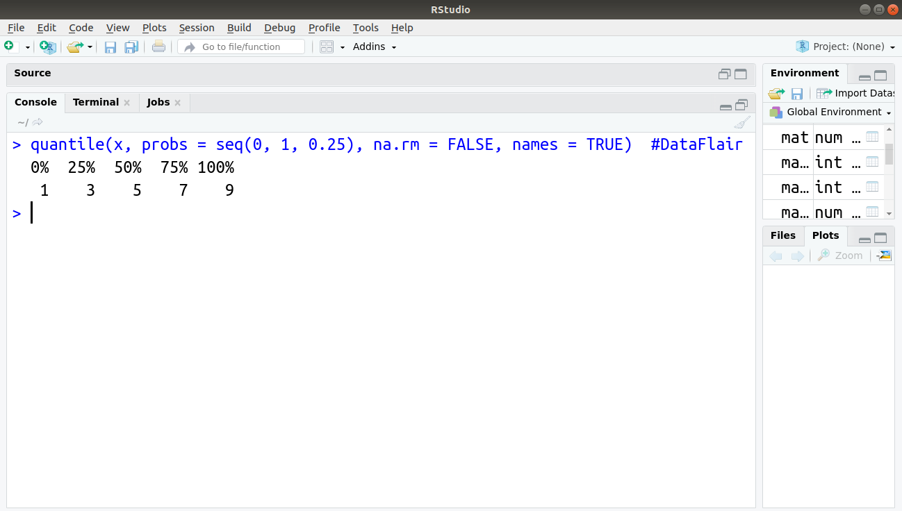
quantile(x, probs = seq(0, 1, 0.25), na.rm = FALSE, names = TRUE)
Output:
X in the command is the data object you wish to examine.
The probs = instruction enables you to select one or several quantiles to display, defaulting to 0, 0.25, and so on. This is what the seq(0, 1, 0.25) command is doing: Setting a start of 0, an end of 1, and a step of 0.25. This is the same as c(0, 0.25, 0.5, 0.75, 1). The names = instruction tells R if it should display the name of the quantiles produced.
Explore major functions to organise your data in R Data Reshaping Tutorial
R Cumulative Statistics
Cumulative statistics in R is applied sequentially to a series of values. It is used to track the interest received on an investment.
When data involves interest payments received then the cumulative sum would be a running total that includes the interest part of each payment. The commands that calculate cumulative statistics are of two types:
- Simple Cumulative Commands – Need only the name of the object.
- Complex Cumulative Commands – Should be used in combination with other commands to produce more useful results.
Any queries in R descriptive statistics concept till now? Share your doubts in the comment section below.
Simple Cumulative Commands in R
These are the commands that need only the name of the object. Cumulative commands produce an accurate result when applied to a vector of character data. However, if applied on character data, they give error populated as a list of NA items.
If the numeric vector contains NA, the cumulative command will work till first NA and thereafter give all result as NA.
Below are some commands that return cumulative values:
- Cumsum(x) – The cumulative sum of a vector.
- Cummax(x) – The cumulative maximum value.
- Cumin(x) – The cumulative minimum value.
- Cumprod(x) – The cumulative product.
Let us see this with an example:
A vec is a vector comprising of values 3, 5, 7, 5, 3, 2 and 6. In order to find its cumulative sum:
> #Author DataFlair
> vec = c(3,5,7,5,3,2,6)  #Creating vector
> cumsum(vec)
> cummax(vec)
> cummin(vec)
> cumprod(vec)
Output:

Now, lets quickly jump to R complex cumulative commands in this R descriptive statistics tutorial.
R Complex Cumulative Commands
Cumulative commands should be used with other commands to produce additional useful results; for example, the running mean.
The basic arithmetic mean is the sum divided by the number of observations. You require the cumulative number of observations to obtain the cumulative sum.
The seq() command can ease cumulative calculations. The index can be created from a sample of numeric values. The main purpose of the command is to generate sequences of values.
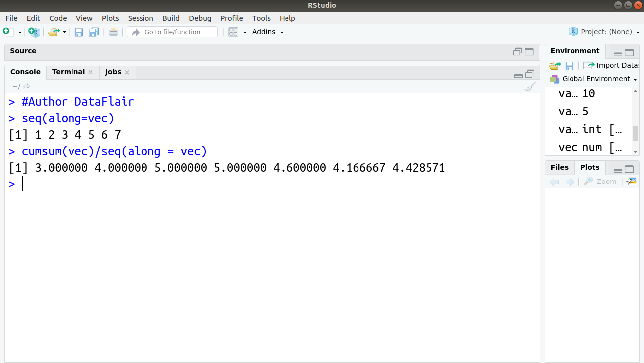
Let us see the use of seq() command on data2 above. We can also combine cumsum() and seq() command as follows:
> #Author DataFlair
> seq(along=vec)
> cumsum(vec)/seq(along = vec)
Output:
Wait! Have you checked – Numeric and Character Functions in R
Descriptive Statistics in R for Data Frames
Summarizing single vector of data is a simple and straight-forward process. You can directly apply the summarizing command to get results. However complicated data objects are demanding and require some amount of workaround.
Let us see a few generic commands for data frames as below:
- Max(frame) – Returns the largest value in the entire data frame.
- Min(frame) – Returns the smallest value in the entire data frame.
- Sum(frame) – Returns the sum of the entire data frame.
- Fivenum(frame) – Returns the Tukey summary values for the entire data frame.
- Length(frame)- Returns the number of columns in the data frame.
- Summary(frame) – Returns the summary for each column.
You can extract a single vector from your data frame and perform a summary of some sort on it. This approach will not work for rows of data frames.
R Special Summary Commands
There are two types of special summary commands:
- Row Summary Commands – Applied to work with row data. Two commands here are rowmeans() and rowsums().
- Column Summary Commands – Also, applied to work with row data but the two commands here are colmeans() and colsums().
R Row Summary Commands
The row summary commands in R work with row data. rowmeans() command gives the mean of values in the row while rowsums() command gives the sum of values in the row.
Suppose that we have the dataframe that represents scores of a quiz that has five questions. Here, each student is represented in a row and each column denotes a question. There are two categories 1 and 0 that correspond to correct and incorrect respectively.
| Q1 | Q2 | Q3 | Q4 | Q5 |
| 0 | 0 | 0 | 1 | 1 |
| 0 | 1 | 0 | 1 | 0 |
| 0 | 1 | 0 | 1 | 1 |
| 0 | 0 | 1 | 1 | 0 |
| 1 | 1 | 1 | 1 | 1 |
#Author DataFlair
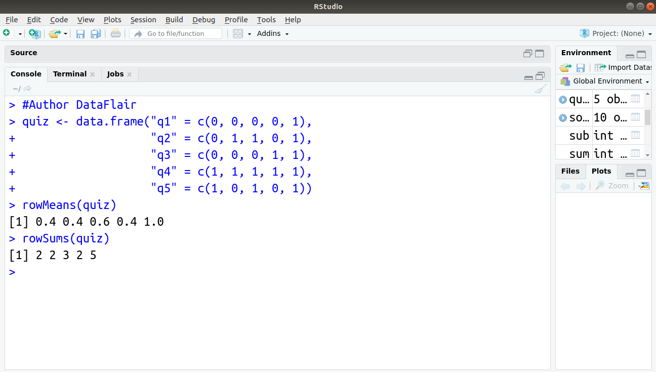
quiz <- data.frame("q1" = c(0, 0, 0, 0, 1),
"q2" = c(0, 1, 1, 0, 1),
"q3" = c(0, 0, 0, 1, 1),
"q4" = c(1, 1, 1, 1, 1),
"q5" = c(1, 0, 1, 0, 1))
rowMeans(quiz)
rowSums(quiz)Output:
You must have a look at R Data Frame Concept
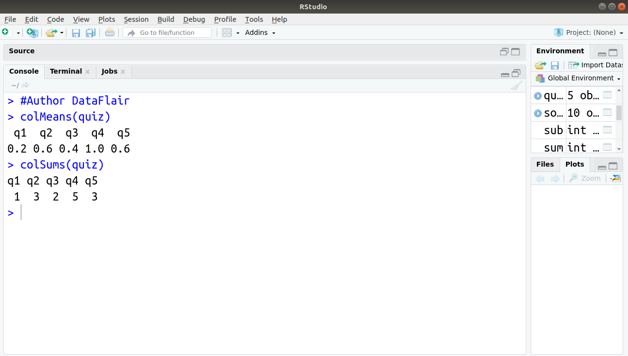
Column Summary Commands in R
These R commands work with column data.
> #Author DataFlair
> colMeans(quiz)
q1 q2 q3 q4 q5
0.2 0.6 0.4 1.0 0.6
> colSums(quiz)
q1 q2 q3 q4 q5
1 3 2 5 3
Output:
The apply() Command in R for Summaries
Colmeans() and rowsums() commands are quick alternative to a more general command apply().
The apply() command enables applying a function to the rows or columns of a matrix or data frame. Depending on what function you specify when using the apply command, you will get back either a vector or a matrix. The general form of the command is:
apply(X, MARGIN, FUN, ...)
x specifies the matrix or data frame.
MARGIN command uses either 1 or 2, where 1 is for rows and 2 is for columns. You replace the FUN part with your command (the function you want to apply).
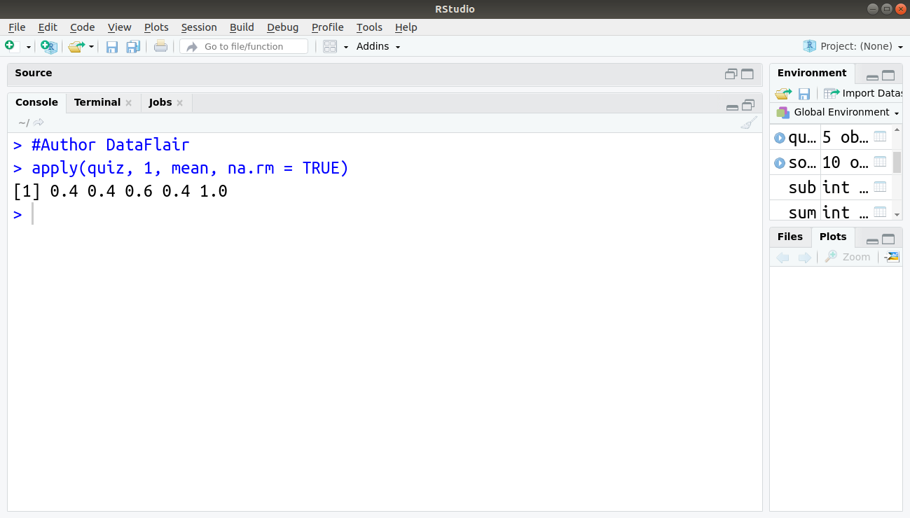
You can also add additional instructions if they are appropriate to the command/function you are applying. For example – You might add the na.rm = TRUE instruction as follows:
> #Author DataFlair
> apply(quiz, 1, mean, na.rm = TRUE)
Output:
Gain expertise in apply() and supply() functions from R Matrix Functions Tutorial
Descriptive Statistics in R for Matrix Objects
A matrix may look like a data frame but is not. In a matrix object, data split into rows and columns though it is a single vector.
With data frame, you can use $ to extract data but you cannot extract parts of a matrix using $. You can use the square brackets to retrieve information of any row or column.
In this section, we will create our matrix ‘mat’ of 5 rows and 6 columns as follows:
mat <- matrix(rnorm(30), nrow=5, ncol=6)
mean(mat[,2])
mean(mat[2,])
Output:
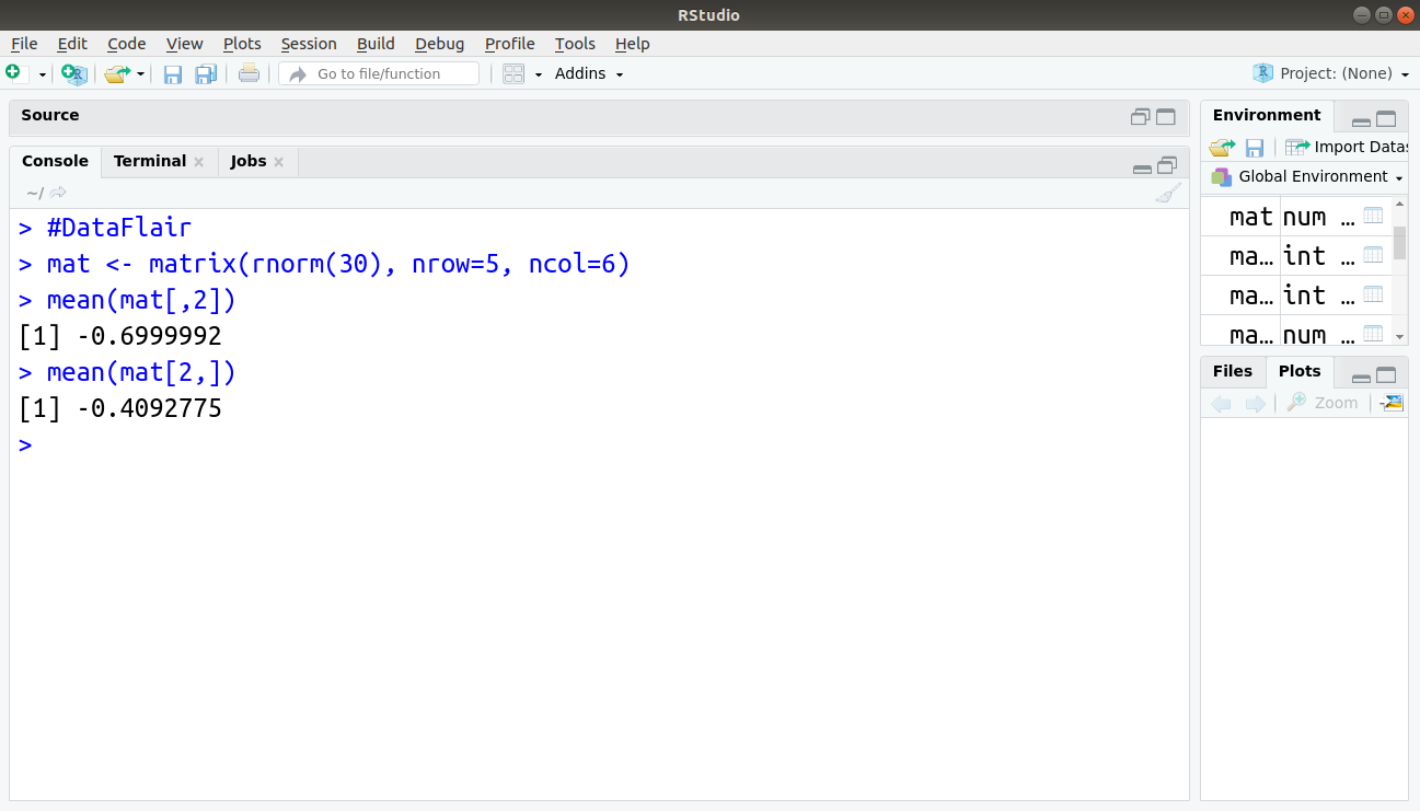
The first example returns the mean for the second column, while the next example returns the mean for the second row using colmeans() and rowsums() commands as the before one is also applicable to matrices.
The apply() command also works equally well for a matrix as it does for data frame objects. An example of using apply() command for data frames is as follows:
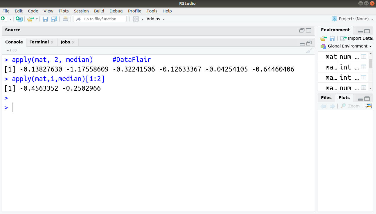
> apply(mat, 2, median)
In this case, we extract the median values for the columns of the matrix. Customizing of the result is also possible for specific elements of data.
One can append the square brackets after the command for customizing the result for specific elements of data.
apply(mat,1,median)[1:2]
Output:
Summary
In this tutorial of R descriptive statistics, we understood its whole concept and also learned about different R commands covered under the descriptive statistics. We hope the examples used for implementing the commands was understandable to you.
Next topic that I would recommend you to complete is Introduction to R Contingency Tables
If you found any difficulty in understanding the descriptive statistics in R, share your queries in the comment section below.
You give me 15 seconds I promise you best tutorials
Please share your happy experience on Google


it was very very useful